Download
1 / 8
80 likes | 94 Vues
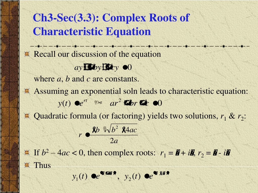
Ch3-Sec(3.3): Complex Roots of Characteristic Equation. Recall our discussion of the equation where a , b and c are constants. Assuming an exponential soln leads to characteristic equation: Quadratic formula (or factoring) yields two solutions, r 1 & r 2 :

E N D
Ch3-Sec(3.3): Complex Roots of Characteristic Equation • Recall our discussion of the equation where a, b and c are constants. • Assuming an exponential soln leads to characteristic equation: • Quadratic formula (or factoring) yields two solutions, r1 & r2: • If b2 – 4ac < 0, then complex roots: r1 = + i, r2 = - i • Thus
Euler’s Formula; Complex Valued Solutions • Substituting it into Taylor series for et, we obtain Euler’s formula: • Generalizing Euler’s formula, we obtain • Then • Therefore
Real Valued Solutions • Our two solutions thus far are complex-valued functions: • We would prefer to have real-valued solutions, since our differential equation has real coefficients. • To achieve this, recall that linear combinations of solutions are themselves solutions: • Ignoring constants, we obtain the two solutions
Real Valued Solutions: The Wronskian • Thus we have the following real-valued functions: • Checking the Wronskian, we obtain • Thus y3 and y4 form a fundamental solution set for our ODE, and the general solution can be expressed as
Example 1 (1 of 2) • Consider the differential equation • For an exponential solution, the characteristic equation is • Therefore, separating the real and imaginary components, and thus the general solution is
Example 1(2 of 2) • Using the general solution just determined • We can determine the particular solution that satisfies the initial conditions • So • Thus the solution of this IVP is • The solution is a decaying oscillation
Example 2 • Consider the initial value problem • Then • Thus the general solution is • And • The solution of the IVP is • The solution is displays a growing oscillation
Example 3 • Consider the equation • Then • Therefore • and thus the general solution is • Because there is no exponential factor in the solution, so the amplitude of each oscillation remains constant. The figure shows the graph of two typical solutions