Download

1 / 243
2.43k likes | 2.44k Vues
This study aims to show that the perfect matching problem in bipartite graphs can be solved in the Quasi-NC complexity class, using polylogarithmic depth bounded uniform circuits.

E N D
Bipartite Graph Perfect Matching is in quasi-NC Ron Sinai – Eliran Abdu – AlonGromakov
NC • “In complexity theory, the class NC ("Nick's Class") is the set of decision problems decidable in polylogarithmic time on a parallel computer with a polynomial number of processors.” In other words, a problem is in NC if there exist constants c and k such that it can be solved in time O() using O() parallel processors.
NC • “In complexity theory, the class NC ("Nick's Class") is the set of decision problems decidable in polylogarithmic time on a parallel computer with a polynomial number of processors.” In other words, a problem is in NC if there exist a series of uniform circuits of poly-logarithmic depth and polynomial size
NCi is the class of decision problems decidable by uniform boolean circuits with a polynomial number of gates of at most two inputs and depth O(login), or the class of decision problems solvable in time O(login) on a parallel computer with a polynomial number of processors.
RNC RNC is the set of problems that are in NC, with the extension of access to randomness.
Quasi-NC the class of problems which have uniform circuits of quasi-polynomial size (c>1) and poly-logarithmic depth O(). Here, uniformity means that local queries about the circuit can be answered in poly-logarithmic time. Quasi-
Bipartite Graph Perfect Matching is in QUASI-NC • GOAL: show that for bipartite graphs, the perfect matching problem is in quasi-nc.
Bipartite Graph Perfect Matching is in QUASI-NC • GOAL: show that for bipartite graphs, the perfect matching problem is in quasi-nc. • So far, best bound for poly logarithmic depth bounded uniform circuits:
Bipartite Graph Perfect Matching is in QUASI-NC • GOAL: show that for bipartite graphs, the perfect matching problem is in quasi-nc. • So far, best bound for poly logarithmic depth bounded uniform circuits: • De-Randomization: solving a problem that uses random bits with almost no usage of random bits (complete de-randomization – O(log(n)) random bits)
Bipartite Graph Perfect Matching is in QUASI-NC • GOAL: show that for bipartite graphs, the perfect matching problem is in quasi-nc. • So far, best bound for poly logarithmic depth bounded uniform circuits: • De-Randomization: solving a problem that uses random bits with almost no usage of random bits (complete de-randomization – O(log(n)) random bits) • Parallelization: solving a problem in parallel by using multiple processors
Bipartite Graph Perfect Matching is in QUASI-NC • GOAL: show that for bipartite graphs, the perfect matching problem is in quasi-nc. • So far, best bound for poly logarithmic depth bounded uniform circuits: • De-Randomization: solving a problem that uses random bits with almost no usage of random bits (complete de-randomization – O(log(n)) random bits) • Parallelization: solving a problem in parallel by using multiple processors We will try to solve the problem of finding a perfect matching in a graph by de-randomizing the isolation lemma, and parallel computation.
Lemma 1.1 (Isolation Lemma) For a graph G(V, E), let w be a random weight assignment, where edges are assigned weights chosen uniformly and independently at random from{1, 2, . . . , 2|E|}. Then w is isolating with probability ≥ 1/2.
Lemma 1.1 (Isolation Lemma) For a graph G(V, E), let w be a random weight assignment, where edges are assigned weights chosen uniformly and independently at random from{1, 2, . . . , 2|E|}. Then w is isolating with probability ≥ 1/2. We look at the elements We choose a weight Probability ½
RNC algorithm for Search-PM (Mulmuley, Vazirani & Vazirani) First, a reminder: • A graph G is called bipartite if there exists a partition V = L U R of the vertices, such that all edges are between vertices of L and R.
RNC algorithm for Search-PM (Mulmuley, Vazirani & Vazirani) First, a reminder: • A graph G is called bipartite if there exists a partition V = L U R of the vertices, such that all edges are between vertices of L and R. • In graph G(V,E), a matching M is a subset of edges with no two edges sharing an endpoint.
RNC algorithm for Search-PM (Mulmuley, Vazirani & Vazirani) First, a reminder: • A graph G is called bipartite if there exists a partition V = L U R of the vertices, such that all edges are between vertices of L and R. • In graph G(V,E), a matching M is a subset of edges with no two edges sharing an endpoint. • Perfect Matching – a matching which covers every vertex.
RNC algorithm for Search-PM (Mulmuley, Vazirani & Vazirani) First, a reminder: • A graph G is called bipartite if there exists a partition V = L U R of the vertices, such that all edges are between vertices of L and R. • In graph G(V,E), a matching M is a subset of edges with no two edges sharing an endpoint. • Perfect Matching – a matching which covers every vertex. • For any weight w: on the edges, the weight of M is defined to be
RNC algorithm for Search-PM (Mulmuley, Vazirani & Vazirani) First, a reminder: • A graph G is called bipartite if there exists a partition V = L U R of the vertices, such that all edges are between vertices of L and R. • In graph G(V,E), a matching M is a subset of edges with no two edges sharing an endpoint. • Perfect Matching – a matching which covers every vertex. • For any weight w: on the edges, the weight of M is defined to be • A perfect matching exists in G only if |L| = |R| =
RNC algorithm for Search-PM (Mulmuley, Vazirani & Vazirani) Let G be a bipartite graph with vertex partitions and weight function w. Consider the following matrix A associated with G: A(I,j) =
RNC algorithm for Search-PM (Mulmuley, Vazirani & Vazirani) Let G be a bipartite graph with vertex partitions and weight function w. Consider the following matrix A associated with G: A(I,j) = The algorithm computes the determinant of A.
W)E( כחול: 1שחור: 2אדום: 3סגול: 4 4 W=6 1 W=3 4 1 5 2 2 W=6 3 6 5 W=8 4 5 6 1| 2| 3| A: 3 W=7
RNC algorithm for Search-PM (Mulmuley, Vazirani & Vazirani) Sgn(M) – the sign of the corresponding permutation
RNC algorithm for Search-PM (Mulmuley, Vazirani & Vazirani) Sgn(M) – the sign of the corresponding permutation Clearly, if G has no PM, then det(A) = 0. If G does contain a PM, det(A) can still calculate to zero (cancellations)
RNC algorithm for Search-PM (Mulmuley, Vazirani & Vazirani) Sgn(M) – the sign of the corresponding permutation Clearly, if G has no PM, then det(A) = 0. If G does contain a PM, det(A) can still calculate to zero (cancellations) Motivation: We need a weight assignment that will ensure det(A)≠ 0 i.f.f G has PM
Isolating Weight Function For a graph G(V,E), a weight assignment w is called isolating if the minimum weight PM in G is unique, if one exists.
RNC algorithm for Search-PM (Mulmuley, Vazirani & Vazirani) Sgn(M) – the sign of the corresponding permutation Clearly, if G has no PM, then det(A) = 0. If G does contain a PM, det(A) can still calculate to zero (cancellations) Motivation: We need a weight assignment that will ensure det(A) ≠0 i.f.fiff G has PM
RNC algorithm for Search-PM (Mulmuley, Vazirani & Vazirani) Sgn(M) – the sign of the corresponding permutation Clearly, if G has no PM, then det(A) = 0. If G does contain a PM, det(A) can still calculate to zero (cancellations) Motivation: We need a weight assignment that will ensure det(A) ≠ 0 iff G has PM • If G has a PM and w is isolating then det(A) ≠ 0.
RNC algorithm for Search-PM (Mulmuley, Vazirani & Vazirani) Sgn(M) – the sign of the corresponding permutation Clearly, if G has no PM, then det(A) = 0. If G does contain a PM, det(A) can still calculate to zero (cancellations) Motivation: We need a weight assignment that will ensure det(A) ≠ 0 iff G has PM • If G has a PM and w is isolating then det(A) ≠ 0. Note: even if w is isolating, we still need to build A as before by assigning A(I,j) = this way we won’t get cancellations (otherwise we can still get them) – because no 2 PM’s of same minimal weight, so well have 1 at least remaining.
RNC algorithm for Search-PM (Mulmuley, Vazirani & Vazirani) Given that w is isolating: G has a PM I.F.F det(A) ≠ 0. Proof: => If G has a PM and w is an isolating weight assignment then there exists a perfect matching M with a minimal weight W and it is unique (def).Therefore:
RNC algorithm for Search-PM (Mulmuley, Vazirani & Vazirani) Given that w is isolating: G has a PM I.F.F det(A) ≠ 0. Proof: => If G has a PM and w is an isolating weight assignment then there exists a perfect matching M with a minimal weight W and it is unique (def).Therefore: because w is isolating, looking at as a binary number among all the other powers of two – it represents the LSB 1, and every other operand has a 0 in that coordinate of it’s binary representation. Therefore (Negation in 2’s complement of every element is the same element)
RNC algorithm for Search-PM (Mulmuley, Vazirani & Vazirani) Given that w is isolating: G has a PM I.F.F det(A) ≠ 0. Proof:<= Let’s assume det(A) ≠ 0 then one of the operands in the sum had to be non zero, therefore G has a PM.
RNC algorithm for Search-PM (Mulmuley, Vazirani & Vazirani) Construction of the Perfect Match: Given an isolating weight assignment: we would like to construct -min weight Perfect Matching.Find the largest power of 2 that divides det(A) – O(log(n)) (in parallel)
RNC algorithm for Search-PM (Mulmuley, Vazirani & Vazirani) Construction of the Perfect Match: Given an isolating weight assignment: we would like to construct -min weight Perfect Matching.Find the largest power of 2 that divides det(A) – O(log(n)) (in parallel). That would be the weight of the min weight perfect match (
RNC algorithm for Search-PM (Mulmuley, Vazirani & Vazirani) Construction of the Perfect Match: Given an isolating weight assignment: we would like to construct -min weight Perfect Matching.Find the largest power of 2 that divides det(A) – O(log(n)) (in parallel). That would be the weight of the min weight perfect match ( From the example: we had:
RNC algorithm for Search-PM (Mulmuley, Vazirani & Vazirani) Construction of the Perfect Match: Given an isolating weight assignment: we would like to construct -min weight Perfect Matching.Find the largest power of 2 that divides det(A) – O(log(n)). That would be the weight of the min weight perfect match ( • For every edge e, compute the determinant of If the result does not contain then e is in (Based on determinant calculation - every minor in the calculation represents an edge)
RNC algorithm for Search-PM (Mulmuley, Vazirani & Vazirani) Construction of the Perfect Match: Given an isolating weight assignment: we would like to construct -min weight Perfect Matching.Find the largest power of 2 that divides det(A) . That would be the weight of the min weight perfect match ( • For every edge e, compute the determinant of If the result does not contain then e is in (Based on determinant calculation - every minor in the calculation represents an edge) • Doing that in parallel for all edges in G we can find the required PM.
RNC algorithm for Search-PM (Mulmuley, Vazirani & Vazirani) We saw in lemma 1.1 that the Isolation Lemma delivers the isolating weight assignment with high probability. Moreover, the weights chosen by the Isolation Lemma are polynomiallybounded. Therefore, the entries in matrix A have polynomially many bits. This suffices to compute the determinant in . Hence, also the construction is in . Put together, this yields an RNC-algorithm for Search-PM (use of random bits).
De-Randomizing the Isolation Lemma First Try: Let E = {and define Then w is clearly isolating (different weight for every matching).Cannot compute det(A) efficiently, because entries are too big.
De-Randomizing the Isolation Lemma First Try: Let E = {and define Then w is clearly isolating (different weight for every matching).Cannot compute det(A) efficiently, because entries are too big. Before: was chosen randomly and uniformly from (and each entry was Now: Each entry in A will be This takes exponentially many bits.
De-Randomizing the Isolation Lemma Goal: deterministically assign weights such that w is isolating.
Circulation Let C = < be a cycle in G with edges given in cyclic order (k is even as G is bipartite). Definition – Nice Cycle:A cycle C in G is called NICE if after removing C from G, G still has a perfect matching.
Circulation Let C = < be a cycle in G with edges given in cyclic order (k is even as G is bipartite). Definition – Nice Cycle:A cycle C in G is called NICE if after removing C from G, G still has a perfect matching. • In other words, a nice cycle can be obtained from the symmetric difference of two perfect matchings. Note that a nice cycle is always an even cycle.
Circulation Claim: Cycle is NICE I.F.F it is a symmetric difference between two P.M’s.
Circulation Claim: Cycle is NICE I.F.F it is a symmetric difference between two P.M’s. Lets assume a cycle c is NICE. Then if we remove it from the graph we still have a PM. Lets denote C by . Now by taking every second edge, we build a PM:
Circulation Claim: Cycle is NICE I.F.F it is a symmetric difference between two P.M’s. Lets assume a cycle c is NICE. Then if we remove it from the graph we still have a PM. Lets denote C by . Now by taking every second edge, we build a PM: We add back to the graph. Now, since C is a series of vertices, . We take and put it back to G adding vertices and connecting them.
Circulation Claim: Cycle is NICE I.F.F it is a symmetric difference between two P.M’s. Lets assume a cycle c is NICE. Then if we remove it from the graph we still have a PM. Lets denote C by . Now by taking every second edge, we build a PM: We add back to the graph. Now, since C is a series of vertices, . We take and put it back to G adding vertices and connecting them. Doing that for every second edge of C, we end up adding each of the vertices from the cycle back to the graph, connecting every two (one from L one from R) with an edge, when no two edges share an endpoint. Hence: we get a perfect matching in G.
Circulation Claim: Cycle is NICE I.F.F it is a symmetric difference between two P.M’s. We got 2 PM’s in G, so that every even edge of C is in and every odd edge is in . Therefore – C is a cycle that contains all edges of that are not in and all edges that are in that are not in . Hence: a symmetric difference between two PM’s.
Circulation Claim: Cycle is NICE I.F.F it is a symmetric difference between two P.M’s. Lets assume C is a cycle that is a symmetric difference between and Looking at all the edges and vertices that are in G\C we find that all of those are common to . Since both of them are PM’s, those edges and vertices form a PM in G\C.