Download
1 / 46
460 likes | 571 Vues
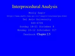
Interprocedural Control Dependence. James Ezick and Kiri Wagstaff CS 612 May 4, 1999. Outline. Motivation Some essential terms Constructing the interprocedural postdominance relation Answering interprocedural control dependence queries Future work. Motivation.

E N D
Interprocedural Control Dependence James Ezick and Kiri Wagstaff CS 612 May 4, 1999
Outline • Motivation • Some essential terms • Constructing the interprocedural postdominance relation • Answering interprocedural control dependence queries • Future work
Motivation • As we have seen in class the Roman Chariots formulation for intraprocedural control dependence (Pingali & Bilardi) has allowed control dependence queries to be answered in (optimal) time proportional to the output size. • We seek to extend that work to cover control flow graphs representing multiple procedures without the need for fully cloning each function.
How would that make the world better? • Recall that control dependence (conds) is the same as the edge dominance frontier relation of the reverse graph. • Recall that the dominance frontier relation is used in the construction of SSA form representations. • If we could build this representation faster it would allow us perform a wide range of code optimizations in a more uniform and more efficient manner.
Valid Paths - Context Sensitive Analysis • Valid path: A path from START to END in which call and return edges occur in well-nested pairs and in which these pairs correspond to call sites and the return sites specific to these call sites. START a F b c d This is intended to exactly capture our intuition of a call stack. END
Other Terms • Node winterprocedurally postdominates v if every valid path from v to end contains w. • Node w is ipcontrol dependent on edge (u v) if • w ip postdominates v • w does not strictly ip postdominate u We notice immediately that these definitions are completely analogous to their intraprocedural counterparts - they however incorporate the notion of valid paths.
First postdominence, then the world! As the definitions suggest there is a tight relationship between control dependence and postdominance. To compute control dependence we first would like to compute postdominance subject to the following criteria: • We minimize cloning to the fullest possible extent. • We are able to parallelize the process. (One function - one thread). • We can deal with all common code constructs (including recursion).
Computing Postdominance • In the intraprocedural case every path through the control flow graph is a valid path and the resulting postdominance relation is a tree. • Algorithms exist to produce this tree which run in time linear in the size of the control flow graph (Rodgers, et al.). • The introduction of non-valid paths into the CFG breaks this property - the transitive reduction is now a DAG.
How is this done today? • We use iterative methods and context sensitive flow analysis to compute postdominance and control dependence. • This involves keeping a table of inputs and outputs. • Convergence occurs due to the finite nature of the table but it is not guaranteed to occur quickly.
General Description • First, we do a generalized form of dataflow analysis in which each procedure acts as a single block box transition function. • By keeping a table of inputs and outputs of this function for each procedure we gain efficiency and can detect termination. • After the interprocedural relationships are understood - we compute the intraprocedural info for each procedure in the usual way.
Where we break down Control Flow Graph Postdominance DAG End Start L Start F-start A F-a G-end F-end J Call F K Call G B C F-end G-a F-a Ret F Ret G E D G-start F-start Call G Call F I H G-start Ret G Ret F J K G-a H I L G-end E D End B C Notice the existence of an invalid path: Start-A-B-(F-Start)-(F-a)-(F-end)-K-L-End A
So What? • We could ignore the invalid paths and claim that we are being “conservative”. • However, if we do this we lose the fact that A is postdominated by both F and G - this is vital information that we can’t sacrifice and still expect to be able to compute control dependence. • We need to construct this DAG in its full form.
Observations • We notice that the postdominance relations for F and G are subgraphs of the entire postdominance relation. • This begs the question - Can we simply compute the postdominance relation with place-holders for F and G and then simply splice the F and G graphs in later? • What information would we need to do this?
First Attempt • Is it enough to simply know the two nodes that “bookend” all the calls to a specific function? Start Start End A A D Start B C Call F Call F E G Ret F H Call F Call F H I B I C G Ret F E Ret F I Ret F H E G B C A D D End End We notice that these two distinct control flow graphs produce the same postdominance DAG minus the presence of the F subgraph. Further, [A,D] bookends the calls to F in each case.
Defeat! • Clearly, this technique fails to capture the fact that in the first case the F subgraph should postdominate both B and C whereas in the second case it should not. • Conclusion: we need to know more than which link to break - we need to know what to do with the ancestors of the destination.
Correct Solutions after Splicing Case I Case II End End Start D Start D H I H I B C E G E G F F B C A A We need more information than which connection to break to accurately do this splice.
What do we need to know? • We can think of a tree or a DAG as a representation of a partial order. Specifically we can think of the postdominance relation as a partial order since it is reflexive, anti-symmetric and transitive. • Given this insight, we see that we need to inject the F subgraph into the partial order. Simply knowing two bounds is not enough to do this.
It gets worse • In the example provided we only needed to place B & C - singleton ancestors of D. In fact we can build CFGs where we have arbitrarily complex subgraphs feeding into D. Z D X Y We want to “splice” F in between D and A. F W U V A
100,100 90,90 100,100 100,100 • In order to inject F into the partial order we must also inject F into every path from a terminal to D. 90,90 70,70 50,80 50,80 F 95,95 95,5 90,90 F F 72,78 65,45 70,70 60,60 40,75 70,70 50,80 40,75 65,45 60,60 0,0 65,45 0,0 0,0 60,60 40,75 We define the partial order as := (a,b) < (c,d) iff (a<c) and (b<d). Furthermore, determining where to break each path requires a sequence of UPD queries.
Union Postdominance • We say that a set T union postdominates a set S in an interprocedural control flow graph if every valid path from an element of S to end contains an element of T. • In the preceding case we must determine for each element of the subtree if it is union postdominated by all of the calls to a specific function. • This is clearly not promising. • This extends Generalized Dominators (Gupta 92).
OK, so we do that - what then? • Our problems do not end there - consider the following CFG. G-Start Start F-Start H-Start G-A Call G Call H Call F Call H F-B G-C B C G-B H-A Ret G Ret F Ret H G-D D F-A Ret H E H-End I G-E F-End End G-End Control Flow Graph for H Control Flow Graph for Main Control Flow Graph for F Control Flow Graph for G
End • When we splice in and expand the graphs for F and G we get two copies of H! I Start D E G-End A F-End G-E F-B G-B G-D G-A H H G-Start F-A G-C F-Start B C Maybe this isn’t so bad - can’t we just “merge” them somehow?
Oh, it’s bad. • Given the partial postdominance relation all I can recover from it about H is that H should be a child of I. • I don’t know which link from I to break; also I again don’t know what to do with the other children of I. • As with the previous case I can create CFGs that make this arbitrarily complicated. Further I must now do UPD queries over the entire CFG.
Plan “A” is a loser • It is clear that we cannot simply compute these function DAGs independently and then splice them together since the splicing is more expensive than the original computation. • We need to find a way to incorporate the splicing information into the original computation. • In essence we need subgraph “placeholders” for each function.
A New Hope • It is clear that in order to construct the postdominator relation componentwise we need more a priori information. • In essence we need to understand all of the possible call sequences a program segment can initiate - then we let transitivity do the rest. • To that end we introduce the notion of “sparse stubs”.
Sparse Stubs • Given a program for which we want to construct a control flow graph we construct a sparse representation in parallel that captures only calls and branches. • We then use this sparse representation as a “stub” which we inject into the gap between a call and return. • This stub then captures what we need to construct a PDD into which we can inject full subgraphs.
An Example Notice that this captures every possible sequence of calls in the program (starts and ends). Since H is a “terminal function” we can represent it as a singleton. F, G (which are not terminal) cannot be represented this way - else we could not distinguish between “F calls H” and “call F then H”. We can employ similar shortcuts to eliminate “repeated suffixes” (ex. “call F, call G, call F”) In the case of recursion the sparse graph will have a loop from the call back to the start node of the function - but that’s fine. Start G-Start F-Start H H G-End F-End End Sparse Representation
That’s great. What now? • We notice immediately some interesting properties of this sparse graph. First any function that is called multiple times will have multiple representations in this graph - but they are all the same. Build them once and use pointers. • If we inject into the “call gap” of a function the subgraph of the sparse representation between start and end we get a “plug” for the gap.
What about this plug? • We notice that the plug captures exactly all of the valid paths of the program. • Further, it contains enough information to produce in the resulting PDD placeholders for the component functions. • The price of this good fortune is that we now have duplicate nodes in the control flow graph (these however are all start & end nodes).
Union Postdominance • We now have a purely graph theoretic problem for which we need (have?) a good algorithm. • Given a directed graph with a source and sink and a partition of the nodes P - construct the PDD consisting of the elements of the partition. • We have a naïve quadratic algorithm to do this but we are looking at existing algorithms with better performance that solve similar problems.
Can’t we just see an example? Start Start Start B Call G C Call F G-Start F-Start F-Start G-Start B C = + H H Ret G Ret F D H H E G-End F-End I G-End F-End End End D E Control Flow Graph for Main Sparse Representation I End In this case the partition P is the set of singletons with the two H nodes in a single set. CFG ready for UPD Algorithm
Produce the UPDD for each function End Start Given this UPDD and the other UPDDs for F, G & H we use the starts and ends as placeholders to splice them in. In essence, we “pattern match” to construct the full UPDD. (In practice - use pointers.) I Start B C F-Start G-Start H D A E UPD Algorithm H H G-End F-End G-End F-End F-Start G-Start D E B C I Notice that this is a tree - there are no invalid paths! End H appears in this graph only once - in exactly the correct location!
Final Observations • We notice that the only cloning which has occurred related to the functions called - not their functionality • Once the sparse stub graph is constructed the individual UPDD can be constructed independently. • Using pointers - splicing is now constant time. • We can deal with recursion and cyclic calls.
Control Dependence • Node w is control dependent on edge (u v) if • w postdominates v • w does not strictly postdominate u START END a b c d e a e START START a b b b c c e d a c d END Control Flow Graph Postdominator Tree Control Dependence Relation
Queries on Control Dependence • cd(e): set of nodes control dependent on edge e • conds(v): set of edges v is control dependent on • cdequiv(v): set of nodes with same control dependencies as node v a b c d e START a b c Control Dependence Relation
Roman Chariots: cd(e) • Represent cd(e) as an interval on the pdom tree • cd(u v) = [v, END] - [u, END] = [v, parent(u)) • cd(START a) = [a, END) • cd(b c) = [c, e) END a b c d e e START a START b b c d a a c Control Dependence Relation Postdominator Tree
Roman Chariots: conds(v) • Record intervals at bottom endpoints • Variable amounts of caching END END {} e {1} e {} START START b {1,2} b d a a {2} d a a {1} {1} c c {2} {2} No caching Full caching
Roman Chariots: cdequiv(v) • Compute fingerprints for conds sets • size of conds set • lo(conds): lowest node contained in all intervals in conds set • Two conds sets are equal iff fingerprints match
The Interprocedural Case • Postdominance relation is a DAG, not a tree START END j a START b f fe ge call F call G c g fs gs e i d h d h call G call F e i c g j b f END a Control Flow Graph Postdominator DAG
Interprocedural cd Queries • cd(u v) = [v, END] - [u, END] • Tree: linear interval • DAG: many paths! • No simple parent(v) trick (v may have multiple parents) • In fact, we want an all-paths interpretation • Roman Aqueducts! • u is a polluted source, v is a pure source • Emperor: “Which cities still have clean water?”
Intervals on the DAG • To compute cd(u v), need [v, END] - [u, END] • Break [v, END] into aqueducts (linear intervals) • For each aqueduct, is endpoint pollutable (reachable) by u? • If so, replace endpoint with point where flows from u and v merge (LCA(startpoint, u)) • change interval to open instead of closed to ensure exclusion of (polluted) LCA • Then cd(u v) = union of (modified) aqueducts
Example: cd(a b) cd(a b) = [b,b] + [c,d] + [fs,fs) + [e, j) +[gs,gs) = {b,c,d,e} END j START fe ge fs gs e i d h c g b f a Postdominator DAG
Interprocedural conds Queries • Emperor: “Which flows pass through a certain city?” • Search all aqueduct systems for that city • Faster: use variable caching END j START fe ge fs gs e i d h c g b f a Postdominator DAG
Interprocedural cdequiv Queries • Emperor: “I know that one city is polluted. What other cities are similarly affected?” • Compare aqueduct systems for all cities for matches • Faster: apply ‘fingerprint’ approach
Final Observations II • We can compute intervals on the DAG (viewed as Roman Aqueducts) • We have shown procedures for answering interprocedural control dependence queries • We may be able to extend the faster methods from the Roman Chariots approach to the interprocedural case as well
In Conclusion ... • We have demonstrated a foundation on which to build an interprocedural analysis capable of dealing with modern programming constructs without resorting to iteration or extensive cloning. • What lies ahead is to prove this foundation correct and superior to existing techniques with more rigorous proofs and a working implementation. • At this time we are very optimistic about this formulation.