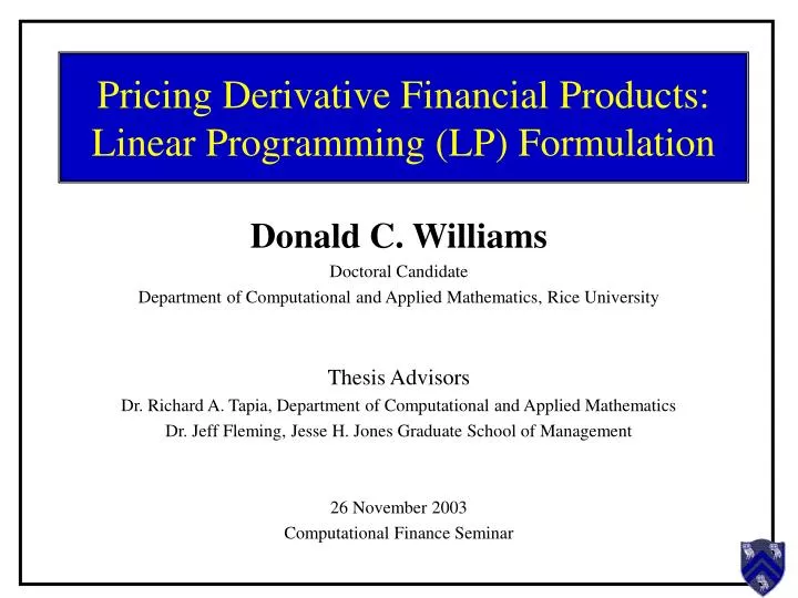
Pricing Derivative Financial Products: Linear Programming (LP) Formulation

1. Pricing Derivative Financial Products: Linear Programming (LP) Formulation Donald C. Williams Doctoral Candidate Department of Computational and Applied Mathematics, Rice University Thesis Advisors Dr. Richard A. Tapia, Department of Computational and Applied Mathematics Dr. Jeff Fleming, Jesse H. Jones Graduate School of Management 26 November 2003 Computational Finance Seminar

2. Outline • Motivation • Nature of Derivative Financial Products • European-style option • Modeling: American-style option • Linear Complementarity Problem • Optimization Framework • LP • Constraints • Concluding Remarks

3. Option Contract Specification Basic Financial Contracts: An American-style option is a financial contract that provides the holder with the right, without obligation, to buy or sell an underlying asset, S, for a strike priceK, at any exercise time where T denotes the contract maturity date. An European-style option is similarly defined with exercise restricted to the maturity date, T .

4. Option Types Two Basic Option Types: A call option gives the holder the right to buy the underlying asset. A put option gives the holder the right to sell the underlying asset.

5. K K ST ST K K ST ST Payoff: Fundamental Constructs Payoff Functions Short position Long position Call Option Put Option

6. Modeling Assumptions • The market is frictionless • e.g., no transaction cost, all market participants have access to any information, borrow and lending rate are equal • No arbitrage opportunities • Asset price follows a geometric Brownian motion • Riskless rate, r, and volatility, , are constant • Option is European-style Classic Black-Scholes Economy:

7. Modeling Building Framework • Define State Variables. Specify a set of state variables (e.g., asset price, volatility) that are assumed to effect the value of the option contract. • Define Underlying Asset Price Process. Make assumptions regarding the evolution of the state variables. • Enforce No-Arbitrage. Mathematically, the economic argument of no-arbitrage leads to a deterministic partial differential equation (PDE) that can be solved to determine the value of the option.

8. Asset Price Evolution Given a constant-variance diffusion approach to asset price changes (i.e., one-factor model of asset price evolution) • where • dW is a standard Browian motion, • μ is the expected return (or drift), and • σ denotes the volatility of asset price returns. The value function V, for an option on an underlying asset that evolves according to dS, satisfies the well-known and celebrated Black-Scholes (1973) parabolic PDE. (cf. Hull (2000))

9. K ST Black-Scholes PDE In the case of European-style options, the value function solves the Black-Scholes equation with appropriate boundary conditions. Initial & Boundary Conditions: (Put Option) IC: BC: Payoff Functions

10. Computational Domain

11. Example: European-Style Put Option Problem Data: S0 = 100; K = 100; T = 0.50; r = 0.05; sigma = 0.25; V(S0,0) = 5.5776 VBS = 5.7910

12. Modeling Basic Question: What changes? American-style contract European-style contract

13. American Option Valuation • Early work focused on discrete dividends and analytic solutions • (1977) Roll • (1979) Geske • (1981) Whaley • When closed-form solutions cannot be derived • (1977) Brennan-Schwartz: Finite-Difference-Method (FDM) • (1978) Brennan-Schwartz: Equivalence of explicit FDM and jump model • (1979) Cox-Ross-Rubinstein: Binomial Pricing Model

14. American Option Valuation • Relaxations of underlying assumption • Stochastic volatility: Heston (1993), Stein-Stein • Deterministic Volatility Function (DVF): Derman-Kani (1994), Dupire (1994), Rubinstein (1994) • Empirical test of DVF: Dumas-Fleming-Whaley (1998) • Jump diffusion process: d’Halluin-Forsyth-Labahn (2003)

15. Modeling No Arbitrage: (put option) Not Optimal to Exercise Early Optimal to Exercise Early

16. Modeling Let: and Then, Continuation Region Exercise Early Region

17. Linear Complementarity Problem (LCP) The American put value function can be expressed as the unique solution to the following LCP: (cf., Dempster-Hutton (1999))

18. Discretized LCP and Equivalent LP Discretized sequence of LCPs: Equivalent sequence of LPs: (cf., Dempster-Hutton-Richards (1998))

19. Observations • The discretized sequence of LCPs can be solved in an iterative manner without using the equivalent formulation as an LP. (ref., Wilmott-Howison-Dewynne (1995)) • However, our desire is to move beyond vanilla option pricing and establish a framework that allows more general economic constraints to be considered.

20. Example: American-Style Put Option Problem Data: S0 = 50.00 K=50.00 T=0.42 r=0.10 sigma=0.40 Grid nodes: 201 Time steps: 100 Time step size: 0.00416667 Discretization: Implicit V(S0,0) = 4.2698 V = 4.24 (control variate, Hull, 4ed, p.418)

21. Idea Consider a 2-factor (or 2-state variable problem) where r is the correlation between the Wiener processes. Employing the 2D version of Ito’s Lemma and no-arbitrage arguments a more general governing B-S PDE is obtained.

22. Ongoing Work Recall the equivalent sequence of LPs: In the context of spread options, consider the constraint

23. Concluding Remarks • Transitioned from American-style option pricing under stochastic volatility to pricing spread option with economic constraints. • Built PDE solver using finite difference. • Presently working to solidify proper numerical implementation of model using LIPSOL to solve the associated LP.