Download

1 / 29
290 likes | 295 Vues
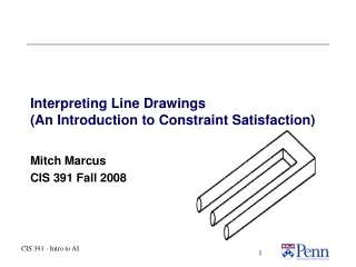
Interpreting Line Drawings. Reprise…. We Interpret Line Drawings As 3D. We have strong intuitions about line drawings of simple geometric figures: We can detect possible 3D objects (although our information is coming from a 2D line drawing).

E N D
Interpreting Line Drawings CSE 140 - Intro to Cognitive Science
Reprise…. CSE 140 - Intro to Cognitive Science
We Interpret Line Drawings As 3D • We have strong intuitions about line drawings of simple geometric figures: • We can detect possible 3D objects (although our information is coming from a 2D line drawing). • We can detect the convexity or concavity of lines in the drawing. • If a line is convex, we have strong intuitions about whether it is an occluding edge. CSE 140 - Intro to Cognitive Science
Guzman’s Theory of Link Inhibition • Guzman (1968) proposed a set of positive and negative cues to the connectivity of objects: • Positive (solid) links suggest that the regions in question correspond to faces of the same object. • Inhibitory (dotted) links suggest that the regions belong to different objects. CSE 140 - Intro to Cognitive Science
Link Inhibition • Guzman’s algorithm was based on link inhibition: • The algorithm should only accept the hypothesis that two regions are parts of the same object, triggered by positive cues from a junction, only in the absence of negative evidence from the junction at the other end. • Guzman’s link inhibition uses the crucial notion of an adjacent pair of junctions. CSE 140 - Intro to Cognitive Science
Guzman’s Link Inhibition Doesn’t Work • The inadequacy of Guzman’s algorithm can be shown by considering CSE 140 - Intro to Cognitive Science
Guzman’s Link Inhibition Doesn’t Work • The inadequacy of Guzman’s algorithm can be shown by considering a cube with a hole in it: CSE 140 - Intro to Cognitive Science
Guzman’s Link Inhibition Doesn’t Work • The inadequacy of Guzman’s algorithm can be shown by considering a cube with a hole in it. • The algorithm perceives this as a cube with a strange floating object above it. • The algorithm is therefore: • Incomplete: It fails to find a possible interpretation for some objects. • Unsound: It attributes impossible interpretations to some objects. CSE 140 - Intro to Cognitive Science
The General-Viewpoint Assumption • This is the assumption that shifts in the position of the viewer do not affect the configuration of the line drawing. • The General-Viewpoint Assumption rules out the possibility of the accidental alignment of image features into a spurious junction. CSE 140 - Intro to Cognitive Science
Huffman/Clowes Junction Labels • Huffman (1971) and Clowes (1971) independently noted that richer information about each junction is necessary, that adding information makes the problem easier. • The problems with Guzman’s link inhibition system could be avoided if a number of distinct connectivity interpretations including convexity information were associated with the junction types. CSE 140 - Intro to Cognitive Science
Convexity Labeling Conventions • A line labeled with a plus (+) indicates that the corresponding edge is convex (angled toward the viewer); • A line labeled with a minus (-) indicates that the corresponding edge is concave (angled away from the viewer); • An arrow indicates an occluding edge. To its right is the body for which the arrow line provides an edge. On its left is space. CSE 140 - Intro to Cognitive Science
The Vocabulary of Huffman/Clowes CSE 140 - Intro to Cognitive Science
“Arrow” Junctions Have 3 Interpretations; “Ls” 6 CSE 140 - Intro to Cognitive Science
“T” Junctions Have 4 Interpretations, “Y” Junctions 5 CSE 140 - Intro to Cognitive Science
Three Arrow Junctions?? A2 A3 A1 (from Winston, Intro to Artificial Intelligence) CSE 140 - Intro to Cognitive Science
Six L Junctions?? L4 L2 L1 L3 L5 L6 CSE 140 - Intro to Cognitive Science
Edge Consistency We now replace Guzman’s link inhibition with edge consistency: Any consistent assignment of labels to the junctions in a picture must assign the same line label to any given line. CSE 140 - Intro to Cognitive Science
An Example of Edge Consistency • Consider an arrow junction with an L junction to the right: • A1 and either L1 or L6 are compatible since they both associate the same kind of arrow with the line. • A1 and L2 are incompatible, since the arrows are pointed in the opposing directions, • Similarly, A1 and L3 are incompatible. CSE 140 - Intro to Cognitive Science
An Example of Edge Consistency II • A1 and L4 are incompatible, since A1 associates an arrow with the line, while L4 associates it with a plus. • A1 and L5 are incompatible, since A1 associates an arrow with the line, while L5 associates it with a minus. CSE 140 - Intro to Cognitive Science
An Example of Edge Consistency III • A2 is compatible with ___? • A3 is compatible with ___? CSE 140 - Intro to Cognitive Science
The Generate and Test Algorithm • Generate all conceivable labelings. • Test each labeling to see whether it violates the edge consistency constraint; throw out those that do. BUT: • Each junction has on average 4.5 labeling interpretations. • If a figure has N junctions, we would have to generate and test 4.5N different labelings. • Thus the Generate and Test Algorithm is O(4.5N). CSE 140 - Intro to Cognitive Science
Is O(4.5N) Bad?? • A picture with 27 junctions, like the devil’s trident) will not be rejected until all 4.527 hypotheses have been rejected, leaving no interpretation. • 4.527 = 433249302231073824.244664378464222 • A computer capable of checking for edge consistency at a rate of 1 hypothesis per microsecond would take about 1 million years to establish that the devil’s trident has no consistent interpretation! CSE 140 - Intro to Cognitive Science
Locally Consistent Search • The Generate and Test algorithm considers too many hypotheses that are simply outright impossible according to the edge consistency constraint. • A better algorithm would exploit locally consistent labelings to construct a globally consistent interpretation: • No junction label would be added unless it was consistent with its immediate neighbors; • If the interpretation could not be continued because no consistent junction label can be added, that interpretation would be abandoned immediately. CSE 140 - Intro to Cognitive Science
Search Trees to the Rescue! We could implement this by constructing a search tree: • Selecting some junction in the drawing as the root. • Label children at the 1st level with all possible interpretations of that junction. • Label their children with possible consistent interpretations of some junction adjacent to that junction. • Each level of the tree adds one more labeled node to the growing interpretation. • Leaves represent either futile interpretations that cannot be continued or full interpretations of the line drawing. CSE 140 - Intro to Cognitive Science
A1 A3 A2 L1 L5 L3 L6 A1 A1 A2 A3 The Top Three Levels of a Search Tree CSE 140 - Intro to Cognitive Science
A1 A3 A2 XX A3 A1 A1 L6 L1 L5 L3 A1 A1 A2 A3 L1 L5 L3 L6 A1 A1 A2 A3 The Fourth Level of the Search Tree X CSE 140 - Intro to Cognitive Science
Breadth-First Search • In breadth-first search, all nodes at the 1st level of the tree are generated, then all nodes at the 2nd, then the 3rd level, and so on until the leaves are reached. • If the average branching factor (the average number of children per node) is B and the depth of the tree is N, then the time complexity of the algorithm is T=O(BN). • We have to keep track of the whole tree as we search, so the space complexity is also S=O(BN). CSE 140 - Intro to Cognitive Science
Depth-First Search • Depth-first search follows one branch of the tree down to its leaf and then backtracks to follow the other branches down to their leaves. • Again, if the average branching factoris B and the depth of the tree is N, then the time complexity of the algorithm is still T=O(BN). • But it requires less space since we only have the hold the junctions on one path from the root with information about which ones were choice points. So its space complexity is only S=O(N). CSE 140 - Intro to Cognitive Science
Another Idea… We are doing somewhat better than the Generate and Test algorithm by not examining useless paths. Nevertheless, we are not fully exploiting the structure of the problem: • Consider a picture with disconnected “islands” (junctions which are not connected by a path along any series of edges). • Both the breadth-first and depth-first methods will explore and re-explore these islands even though they do not interact with the rest of the picture!! This is very wasteful….. CSE 140 - Intro to Cognitive Science