Download
1 / 28
280 likes | 399 Vues
In this lecture, we shall concern ourselves once more with convective mass and heat flows, as we still have not gained a comprehensive understanding of the physics behind such phenomena. We shall start by looking once more at the capacitive field .

E N D
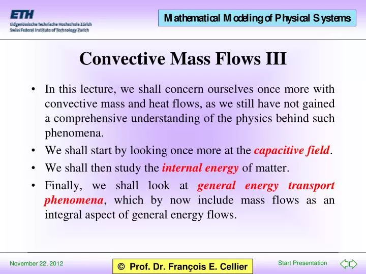
In this lecture, we shall concern ourselves once more with convective mass and heat flows, as we still have not gained a comprehensive understanding of the physics behind such phenomena. We shall start by looking once more at the capacitive field. We shall then study the internal energy of matter. Finally, we shall look at general energy transport phenomena, which by now include mass flows as an integral aspect of general energy flows. Convective Mass Flows III
Capacitive Fields Internal energy of matter Bus-bonds and bus-junctions Heat conduction Volume work General mass transport Multi-phase systems Evaporation and condensation Thermodynamics of mixtures Multi-element systems Table of Contents
Let us briefly consider the following electrical circuit: C2 C1 C2 C3 i1 i3 i2 0 1 0 u1-u2 i3 u2 i2+ i3 i1-i3 i2+i3 u1 i1-i3 u1 u2 i2 u1 u1 u2 0 0 C1 C3 u2 i3 i3 i1 i1 – i3 = C1 · du1 /dt i2 + i3 = C3 · du2 /dt i3 = C2 · (du1 /dt – du2 /dt ) i1 = ( C1 + C2 )· du1 /dt – C2 · du2 /dt i2 = – C2 · du1 /dt + ( C2 + C3 )· du2 /dt Capacitive Fields III
i1 = ( C1 + C2 )· du1 /dt – C2 · du2 /dt i2 = – C2 · du1 /dt + ( C2 + C3 )· du2 /dt C1 C2 C3 Symmetric capacity matrix 0 0 0 1 u1-u2 i3 u2 i2+ i3 u1 i1 i2 ( C1 + C2 ) – C2 – C2 ( C2 + C3 ) ( C2 + C3 ) C2 C2 ( C1 + C2 ) du1 /dt du2 /dt i1-i3 = · i2 u1 u1 u2 0 0 u2 i3 i3 i1 i1 i2 du1 /dt du2 /dt = · C1 C2 + C1 C3 + C2 C3 i2 u1 CF 0 u2 i1 Capacitive Fields IV
Let us consider once more the situation discussed in the previous lecture. C 0 Sf 0 It was no accident that I drew the two capacitors so close to each other. In reality, the two capacitors together form a two-port capacitive field. After all, heat and volume are only two different properties of one and the same material. Cth Cth C S/V 0 1 0 I Volume and Entropy Storage
As we have already seen, there are three different (though inseparable) storages of matter: These three storage elements represent different storage properties of one and the same material. Consequently, we are dealing with a storage field. This storage field is of a capacitive nature. The capacitive field stores the internal energyof matter. MassVolumeHeat The Internal Energy of Matter I
Change of the internal energy in a system, i.e. the total power flow into or out of the capacitive field, can be described as follows : This is the Gibbs equation. Chemical potential · · · · U = T · S - p · V + S mi · Ni Molar mass flow Flow of internal energy i Heat flow Mass flow Volume flow The Internal Energy of Matter II
The internal energy is proportional to the the total mass n. By normalizing with n, all extensive variables can be made intensive. Therefore: Ni ni = n u = s = v = (n·v) + S mi · S V U (n·u) = T · (n· ni ) (n·s) - p · n n n i d d d d d d d d (n·v) - S mi · (n·u) - T · (n· ni ) = 0 (n·s) + p · dt dt dt dt dt dt dt dt i The Internal Energy of Matter III
(n·v) - S mi · (n·u) - T · (n· ni ) = 0 (n·s) + p · i [ ] - S mi · n · - T · + p · i [ u - T · s + p · v - S mi · ni ] + · = 0 i dni dni Flow of internal energy dt dt Finally, here is an explanation, why it was okay to compute with funny derivatives. - S mi · - T · + p · = 0 dv ds du du dv ds dn d d d d i dt dt dt dt dt dt dt dt dt dt dt u - T · s + p · v - S mi · ni Internal energy = 0 i The Internal Energy of Matter IV This equation must be valid independently of the amount n, therefore:
U = T · S - p · V + S mi ·Ni i · · · · · · · U = T · S - p · V + S mi · Ni + T · S - p · V + S mi · Ni i i · · · = T · S - p · V + S mi · Ni i · · · T · S - p · V + S mi · Ni = 0 The Internal Energy of Matter V This is the Gibbs-Duhem equation.
p T V S C C GY q S V CF GY GY · · · p p ni T ni · S C · T · · mi ni mi mi The Capacitive Field of Matter
In the case that no chemical reactions take place, it is possible to replace the molar mass flows by conventional mass flows. In this case, the chemical potential is replaced by the Gibbs potential. Simplifications
The three outer legs of the CF-element can be grouped together. 0 . S T Ø C 3 CF CF C C g q . M p 0 0 Bus-Bond and Bus-0-Junction
CF CF 2 1 3 3 T T 2 Ø 1 Ø 1 . . S S 1 1 . . . DT S T S T S 1 D . D 1 1x 2x 2 S 1 DT 0 2 mGS . mGS DT S 1 2 3 3 HE CF CF 2 1 Once Again Heat Conduction
CF CF 1 2 3 3 p p Ø 1 1 Ø 2 q q . . T S q p T D 1 D S 1x D 2 2x q p D 2 0 GS GS p q D 2 3 3 PVE CF CF 2 1 Volume Pressure Exchange Pressure is being equilibrated just like temperature. It is assumed that the inertia of the mass may be neglected (relatively small masses and/or velocities), and that the equilibration occurs without friction. The model makes sense if the exchange occurs locally, and if not too large masses get moved in the process.
g g The three flows are coupled through RS-elements. 1 . 1 . 2 M M GS T T 1 1 0 . 1 2 . S S 1 2 0 0 Sw Sw This is a switching element used to encode the directionof positive flow. GS mGS mGS p p 1 1 2 q q General Exchange Element I
In the general exchange element, the temperatures, the pressures, and the Gibbs potentials of neighboring media are being equilibrated. This process can be interpreted as a resistive field. r r , S , S 1 1 2 2 CF CF 2 1 3 3 Ø 3 3 Ø RF General Exchange Element II
We may also wish to study phenomena such as evaporation and condensation. HE, PVE, Evaporation, Condensation Ø Ø 3 3 3 3 CF CF gas liq Multi-phase Systems
Mass and energy exchange between capacitive storages of matter (CF-elements) representing different phases is accomplished by means of special resistive fields (RF-elements). The mass flows are calculated as functions of the pressure and the corresponding saturation pressure. The volume flows are computed as the product of the mass flows with the saturation volume at the given temperature. The entropy flows are superposed with the enthalpy of evaporation (in the process of evaporation, the thermal domain loses heat latent heat). Evaporation (Boiling)
Here, a boundary layer must be introduced. Boundary layer CF CF gas gas Rand- schicht 3 3 HE PVE RF 3 3 . Ø Ø HE s S T 3 gas 3 Heat conduction (HE) Volume work (PVE) Condensation and Evaporation Heat conduction (HE) Volume work (PVE) Condensation and Evaporation CF 3 Ø surface . s 3 T S 3 liq HE PVE RF 3 3 Ø Ø HE 3 3 CF CF liq liq Condensation On Cold Surfaces
When fluids (gases or liquids) are being mixed, additional entropy is generated. This mixing entropy must be distributed among the participating component fluids. The distribution is a function of the partial masses. Usually, neighboring CF-elements are not supposed to know anything about each other. In the process of mixing, this rule cannot be maintained. The necessary information is being exchanged. CF CF {M1} {M2} MI 2 {x1} {x2} 1 Thermodynamics of Mixtures
The mixing entropy is taken out of the Gibbs potential. 1 T T . . S S 1 1 p p 1 CF CF q q 12 11 1 1 g1 (T,p) g1(T,p) mix 1 . . M11 x11 M M 1 1 Dg1 T RS . HE PVE . MI M mix DSid 1 1 1 x21 T M21 T . . S S 2 2 p p 1 CF CF q q 22 21 2 2 g2 (T,p) g2(T,p) mix 1 . . M M 2 2 Dg2 T RS . . M mix DSid 2 2 Entropy of Mixing It was assumed here that the fluids to be mixed are at the same temperature and pressure.
T1mix T1 1 . . S S . 1 1 S1 DT1 p1mix p1 1 CF CF q q 12 11 1 1 q1 Dp1 g1(T1,p1) g1(T1,p1) mix 1 . . M1 M . 1 Dg1 M T1mix 1 . RS mRS RS DS1 MI HE PVE 0 T2mix T2 1 . . S S . 2 2 S2 DT2 p2mix p2 1 CF CF q q 22 21 2 q 2 Dp2 It is also possible that the fluids to be mixed are initially at different temperature or pressure values. g2 (T2,p2) g2(T2,p2) mix 1 2 . . M2 M . 2 Dg2 M T2mix 2 . RS mRS RS DS2 0
CF CF 11 21 RF PVE HE 3 3 3 3 3 PVE HE 3 Ø Ø PVE HE 3 3 3 3 RF PVE HE 3 3 3 vertical exchange (mixture) 3 HE PVE Ø HE PVE CF Ø CF 22 12 horizontal exchange (transport) 3 3 3 3 3 3 PVE HE Ø Ø PVE HE RF PVE HE 3 3 3 3 CF CF 13 23 Convection in Multi-element Systems
Gas Gas CF CF HE PVE RF 21 22 3 3 3 3 3 PVE HE 3 Ø Ø PVE HE 3 RF PVE HE 3 3 3 3 + + 3 3 3 Vges 3 Gas Vges 3 Ø Gas CF Ø CF PVE HE PVE HE 11 12 3 3 HE Condensation/ Evaporation PVE HE Condensation/ Evaporation PVE HE Condensation/ Evaporation PVE HE Condensation/ Evaporation PVE phase- boundary 3 3 HE PVE RF 3 3 3 3 3 3 3 Fl. Ø 3 PVE HE CF PVE HE Fl. Ø 3 3 11 CF 12 3 3 {M11,T11,p 11} {M12,T12,p 12} {x21, DSE21, DVE21} 3 3 {x12, DSE12, DVE12} 3 3 PVE HE Ø Ø PVE HE RF PVE HE 3 3 3 3 {x21, DSE21, DVE21} {x22, DSE22, DVE22} Fl. MI Fl. MI CF CF 21 22 1 {M21,T21,p 21} 2 {M22,T22,p 22} Two-element, Two-phase, Two-compartmentConvective System
It may happen that neighboring compartments are not completely homogeneous. In that case, also the concentrations must be exchanged. CFi CFi+1 3 3 HE PVE CE ... ... 3 Ø 3 3 3 Ø Concentration Exchange
Cellier, F.E. (1991), Continuous System Modeling, Springer-Verlag, New York, Chapter 9. Greifeneder, J. and F.E. Cellier (2001), “Modeling convective flows using bond graphs,” Proc. ICBGM’01, Intl. Conference on Bond Graph Modeling and Simulation, Phoenix, Arizona, pp. 276 – 284. Greifeneder, J. and F.E. Cellier (2001), “Modeling multi-phase systems using bond graphs,” Proc. ICBGM’01, Intl. Conference on Bond Graph Modeling and Simulation, Phoenix, Arizona, pp. 285 – 291. References I
Greifeneder, J. and F.E. Cellier (2001), “Modeling multi-element systems using bond graphs,” Proc. ESS’01, European Simulation Symposium, Marseille, France, pp. 758 – 766. Greifeneder, J. (2001), Modellierung thermodynamischer Phänomene mittels Bondgraphen, Diploma Project, Institut für Systemdynamik und Regelungstechnik, University of Stuttgart, Germany. References II