Download
1 / 60
600 likes | 823 Vues
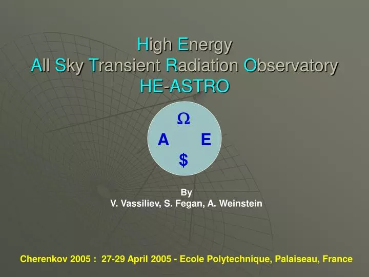
H igh E nergy A ll S ky T ransient R adiation O bservatory HE - ASTRO. W. A. E. $. By V. Vassiliev, S. Fegan, A. Weinstein Cherenkov 2005 : 27-29 April 2005 - Ecole Polytechnique, Palaiseau, France. Scientific Motivations in the realm of GLAST epoch +. Studies of

E N D
High Energy All Sky Transient Radiation ObservatoryHE-ASTRO W A E $ By V. Vassiliev, S. Fegan, A. Weinstein Cherenkov 2005 : 27-29 April 2005 - Ecole Polytechnique, Palaiseau, France
Scientific Motivations in the realm of GLAST epoch + Studies of very high energy transient phenomena In the Universe Studies of the highest energy radiation Galactic sources
Cosmological studies of High Energy Transient Phenomenato determine • Population properties of AGN and GRBs • Redshift evolution of these objects • Redshift evolution of EBL (z=0-6) • Major contributors to EBL (stars, dust, AGN, Population III objects, relic particles, SFR, GFR, IMF, BH accretion histories, supernovae feedback, merger history) • Cosmological magnetic fields and their evolution • High energy properties of space-time
Cosmological Diffuse Background nIn nW m-2 sr-1 l [mm]
Region of strong CDB evolution effect HESS I MAGIC I VERITAS CANGAROO Eg20 GeV – 200 GeV Z<2 (<6) GLAST Universe’s Opacity Redshift Z No CDB Evolution is assumed Energy of g-ray[TeV]
Collecting Area Requirement To resolve ~a few min variability time scale in emission of “Mrk 421-like” AGN placed at Z=1, the collecting area of the observatory must be ~1 km2. E interval g-Rate [GeV] [min-1] 25 - 50 1.3 50 -100 0.7 100 - 200 0.3 3C273 Energetic Quasar Jet by Chandra
Collecting Area Requirement Because the size of the HE-ASTRO, ~1010 cm2, is much larger than the size of the Cherenkov light pool, ~108 cm2, the number of telescopes required is ~102. A Coupling distance: d=80m Area per telescope: A=31/2/ 2 d2 = 5.542x107cm2 Number of telescopes: N=217=3n(n-1) +1; n=9
HE-ASTRO (1st specs) Target Energy Range 20 – 200 GeV Array of 217 telescopes (n=9) Area ~1.0km2 Effective Area ~1.6km2(including boundary events) Detection Rates x 100Hz(flaring nearby AGN) x 1-10Hz(quiescent moderately distant AGN) x few per min(cosmologically distant AGN) Total Cost < $200M(approximate cost of satellite mission) Cost per station < $1M
Problem 1(energy vs area) Although large aperture costly telescopes seem to be favored for low energy range prerequisite, they are incompatible with collecting area constraint due to cost limitations
Ideal Observatory RCR ~3 MHz HE-ASTRO Trade off W A Current IACTAs Solid Angle Requirement Observing Mode: Sky Survey RCR ~300 kHz Un-localized Source RCR ~30 kHz RCR ~3 kHz Known Source
Problems 2 & 3 A requirement of large solid angle coverage, ~p, by the system of a few large aperture telescopes possesses a very difficult engineering problem and costly large aperture secondary optics . Sustaining high data rates in non-distributed system, such as a few large aperture telescopes, is another challenging electronics problem
Collecting Area Data Rate per Telescope FoV per Telescope HE-ASTRO (2nd specs) Energy Range 20–200 GeV Array of 217 telescopes Area ~1.0km2 (~1.6km2) Field of View ~15o FoV area ~177 deg2 Reflector Diameter ~7m Reflector Area ~40 m2 Cost per station < $1M Energy Range Cost per Telescope
GalacticHE Astrophysics Max Acceleration Energy Crab Nebula: 1 g/min > 10 TeV; 2 g/hour > 100 TeV HE pulsars and transients New Phase Space in E, T: New Phase Space in F: If number of sources is a matter of sensitivity in already probed energy domain ,100 GeV – 10 TeV, then collecting area of 1km2 is a figure of merit. Horan & Weekes
Crimea Experiment 1960-1965 HE-ASTRO Challenge Installation at A.E.R.E., Harwell 1962 - Can telescopes be relatively small, have moderately large FoV, be fairly inexpensive, and have differential peak photon detection rate at ~40 GeV?
Understanding Collecting Area Cell Operation Mode QE+Elevation or Dish Size Concept of “IACT-cell” Aharonian at el. Astroparticle Physics 6 (1997) 343-377
For arrival direction For energy estimate ? For CR rejection Important Angular Scales a = ? a = ? Trigger Pixel Size & Trigger Efficiency Image Pixel Size & Reconstruction Efficiency
Challenges • Trigger • Efficiency at low energies (peak of detection rate around 30 – 40 GeV) • High Data rates • Array trigger • Low Cherenkov light level regime • High angular resolution • Background regection efficiency • Engineering & cost issues • Light Sensors • Wide Field of View Optics • Costs
Trigger Pixel Optimization Simulations
Wavelength Response(assumption) Double reflection from aluminized coated mirror Relevant wavelength response window 200 – 400 nm Range of implied QEs 0.5 –1.0 (50% – 100 %) Cherenkov Light Spectrum x (300 nm/l)2 Efficiency Wavelength [nm]
(QE=0.5, D=7m) =(QE=0.25, D=10m) (QE=1.0, D=7m) =(QE=0.5, D=10m) Summary of parameters QE: 0.5 – 1.0 FoV: 10 – 15 degrees Rnsb 0.1 – 1.0 kHz (nth-Nnsb) /Q Trigger Pixel Size [degree] Reflector diameter D=7 m NSB integration window t=20 ns NSB differential flux = 0.4
Lowest trigger threshold(Effects of QE, Rnsb, FoV) Number of photons collected by telescope in trigger pixel in 20 ns from a g-ray shower to trigger pixel of a given size QE=0.5, FoV=15o, Rnsb=0.1 kHz QE=0.5, FoV=10o, Rnsb=0.1 kHz QE=0.5, FoV=15o, Rnsb=1.0 kHz (nth-Nnsb) /Q QE=0.5, FoV=10o, Rnsb=1.0 kHz QE=1.0, FoV=15o, Rnsb=0.1 kHz Effects: 1) QE QE=1.0, FoV=10o, Rnsb=0.1 kHz 2) Rnsb QE=1.0, FoV=15o, Rnsb=1.0 kHz 3) FoV QE=0.5, FoV=10o, Rnsb=1.0 kHz Trigger Pixel Size [degree]
Trigger Efficiency vs Pixel Size(central telescope) El: 3.5 km QE: 1.0, D=7m QE: 0.5, D=10m El: 4.5 km QE: 1.0, D=7m QE: 0.5, D=10m QE: 0.5, D=7m QE: 0.5, D=7m Trigger Efficiency Trigger Pixel Size [degree] Optimum Trigger Sensor pixel size range 0.07o-0.25o Weakly Depends on QE, D, El Parameters: Eg=42 GeV FoV=15o Rnsb=1kHz
Efficiency versus Pixel Size (Array) Array Trigger: Three telescopes above operational threshold p=0.05o p=0.08o p=0.10o p=0.13o Array Parameters: Elevation: 3.5 km QE: 0.5 Reflector: 7 m FoV: 15o p=0.16o p=0.20o Efficiency Efficiency > 50 % p=0.05o – 0.25o for E > 20-30 GeV Photon Energy [GeV]
Single Telescope Trigger Efficiency Diff. spectral index: 2.5 12 GeV Diff. Rate 15 GeV Trigger Efficiency 20 GeV 27 GeV El=4.5km, QE: 1.0, D=7m El=4.5km, QE: 0.5, D=10m El=3.5km, QE: 1.0, D=7m El=3.5km, QE: 0.5, D=10m El=3.5km, QE: 1.0, D=7m El=3.5km, QE: 0.5, D=10m Photon Energy [GeV] Photon Energy [GeV] Effects: 1) “Cell operation” mode 2) Optimum trigger pixel size 3) QE, Reflector Size 4) Elevation 5) Rnsb Parameters: Trigger pixel size: 0.146o Obs. Mode: Un-localized Source (FoV=15o) Rnsb: 1kHz
Single Telescope Trigger Efficiency Diff. spectral index: 2.5 14 GeV Diff. Rate 17 GeV Trigger Efficiency 22 GeV Rnsb: 100kHz Rnsb: 10kHz Rnsb: 1kHz Photon Energy [GeV] Photon Energy [GeV] Effects: 1) “Cell operation” mode 2) Optimum trigger pixel size 3) QE, Reflector Size 4) Elevation 5) Rnsb Parameters: Trigger pixel size: 0.146o Obs. Mode: Known Source (FoV=3.5o)
QE: 0.5 El: 4.5 km, D=7m QE: 0.5 El: 3.5 km, D=7m 30 GeV g triggers 5 telescopes Array trigger El=4.5km, QE: 1.0, D=7m El=4.5km, QE: 0.5, D=10m Trigger Pixel size 0.146o El=3.5km, QE: 1.0, D=7m El=3.5km, QE: 0.5, D=10m Average Number of Telescopes in Trigger Photon Energy [GeV]
Integrated Rate: 32 kHz FoV: 15o Differential CR rates Proton Energy [GeV] Single telescope CR rates
HE-ASTRO (3rd specs) • Array of 217 telescopes • Elevation 3.5km • Telescopes’ coupling distance 80m • Area ~1.0km2 (~1.6km2) • Single Telescope Field of View ~15o • FoV area ~177 deg2 • Reflector Diameter ~7m • Reflector Area ~40 m2 • QE 50% (200-400 nm) • Trigger sensor pixel size 0.146o • Trigger Sensor Size ~31.2cm • NSB rate per Trigger pixel ~3.2 pe per 20 ns • Single Telescope NSB Trigger Rate 1KHz • Energy Range 20–200 GeV • Differential Detection Rate Peak ~30 GeV • Single Telescope CR trigger rate ~ 30 kHz
Event Reconstruction Angular scales
An event g at 42 GeV
Voronoi Diagrams Event 1 (42 GeV) Event 2 (42 GeV)
g-g Separation ScalesImage & NSB g: 21 GeV NSB: 150 g/deg2 g: 42 GeV NSB: 150 g/deg2 Diff. density [Arbitrary] g-g separation [deg] g: 100 GeV NSB: 150 g/deg2 QE: 0.5 Reflector Diameter: 7m Elevation: 3.5 km Trigger pixel size: 0.146o Voronoi Diagram g-g separation scales in Image: 0.01o-0.04o
<d2(qx,qy)>= ∑di2/ ∑1i <p>= ∑pi/ ∑1i Reconstruction Method di , pi uncertainty
Event Reconstruction(arrival direction) <d(qx,qy)>= ∑di2/ ∑1i
21 GeV 42 GeV 100 GeV CR Event containment fraction [1] 4’ 10’ 16’ q radius [deg] Cleaning and arrival direction reconstruction Optimum cut: 4 photons within circle of 0.02o radius
Ln(ng) vs. <p> q < 0.2o No q cut 21 GeV 42 GeV 100 GeV CR Ln(Ng) [1] Mean arrival distance [m] q < 0.05o • The height of shower development • is an effective discriminating factor • which can be utilized within • paradigm of IACT arrays • – e discrimination ? Roadmap to energy estimate!
<p> cut 21 GeV 42 GeV 100 GeV CR 21 GeV 42 GeV 100 GeV Integrated flux [p/deg2/min] Integrated flux [p/deg2/min] Mean arrival distance [m] g containment [fraction] 21 GeV 42 GeV 100 GeV 21 GeV 42 GeV 100 GeV S/N=S/SRT(B) [arbitrary] S/N=S/SRT(B) [arbitrary] Mean arrival distance [m] g containment [fraction]
Event Cleaning CRs Ep=127 GeV
Event Cleaning Photons Eg=42 GeV Eg=100 GeV
Ng vs. <d> Regime: A few hundred photons per event collected by array 21 GeV 42 GeV 100 GeV CR Ng [1] Mean cascade radius <d> [m]
Problem 4(number of pixels) • Both, identification of primary particle and reconstruction of its arrival direction can be accomplished in ~40-50 GeV energy domain. • However, the imaging resolution scales required are in the range 0.01o-0.02o • Optimal pixel size for triggering and imaging differ by a factor of ~10.
Hardware implementation Approach Technologies Data Rates & Array Trigger
Array of MAPMTs Wide field of view optics; possibly of Schmidt type Fine image resolution utilizing CMOS and CCD technology Moderate size primary (6 -7 m) Large aperture Image Intensifier (Electrostatic or MCP) Fast Gated Image Intensifier to reduce NSB 1963 Japan: Suga Italy: ? Russia: ?
The Story of Ground Based g-ray Astronomy (by Jelley & Porter)
Energy range > 1 TeV Readout Event Rate < 1kHz All sky covered with 80 mega pixels in the CMOS sensor arrays Optimized Baker-Nunn optical system with three corrector normal lenses made of acrylic resin and 1 m spherical reflector (spot size less than 1 arcmin, 0.016o, for parallel light rays incident at angles less than 25o). Focal sphere image intensifier, FIIT, of ~60 cm aperture
Focal Plane Instrumentation Fast random access CMOS sensor Image pixel size – 0.0146o Readout image –128 x 128 pixels Readout Image size – 1.875o x 1.875o Readout rate 30-40 kHz Optical or II-based delay Two-mirror reflecting or one-mirror catadioptric optical system X-Y Optical Splitter Gate & Shutter OR X = ∑xi Y = ∑yi Gated Image Intensifier (MCP) (25-40 mm) Gate ~20ns Rep. rate ~40kHz P-43/P-24 , ~2msec Star tracker VETO Trigger Sensor ~8200 pixels with 0.146o Large Aperture Image Intensifier (Electrostatic or MCP) Photon detection efficiency ~50% Fast decay scintillator output screen ~25 ns Primary 7m Fov 15o Array of rate compensated discriminators Slow Control
CMOS Image Sensor HE-ASTRO Image Sensor is not commercially available yet. However, industry is very close to meet specification. High-speed readout is achieved with pipeline and parallel technologies. Parallel processing macro-cell of 32x32 pixels (1024) can be readout with > 500 kHz, and 128 x 128 pixel image (16 macro-cells) with > 30 kHz Micron-MT9M413 1.3-Megapixel CMOS Active Pixel Digital Image Sensor Image pixel size – 0.0146o Readout image –128 x 128 pixels Readout Image size – 1.875o x 1.875o NSB per pixel – 0.032 (20 nsec gate) ADC – 8 bit (S/N improved, 10–>8) Pixel dimension 12mm x 12mm Sensor area – 12.3 mm x 12.3 mm Shutter exposure – a few msec
Ultrafast Imaging DRS technologies Inc. Variety of Ultrafast Cameras for Military applications CCD based 500fps to 100,000,000fps e.g. 350 KHz at 250 x 250 Pixel exposures from 5 nsec limited number of frames 120mm tank gun projectile Photron CMOS based high speed cameras Ultima APX-RS is the world's fastest video camera with 3,000 mega pixel frames per second (fps) or 250,000 fps at reduced resolution FASTCAM-X 1024 PCI is the first system to bring mega-pixel CMOS to your personal computer at usable speeds; capable of operating as fast as 1,000 fps at full 1,024 by 1,024 pixel resolution, or 109,500 fps through ‘windowing‘. Ultima APX-i2 uses a 25mm MCP Gen II image intensifier, directly bonded onto the APX's mega pixel sensor to provide unmatched image quality with 20ns gating. airgun pellet impacting a matchstick
Gated Image Intensifiers Left : C9016-2x Series & Controller Center : C9546 Series Right : C9547 Series Hamamatsu products Commercial products which almost satisfy requirements of resolution, repetition rate, and fast gating exist.