Download
1 / 42
420 likes | 512 Vues
Trees. Tree Basics. A tree is a set of nodes . A tree may be empty (i.e., contain no nodes). If not empty, there is a distinguished node, r, called the root and zero or more non-empty subtrees T 1 , T 2 , T 3 ,….T k , each of whose roots is connected by a directed edge from r.

E N D
Tree Basics • A tree is a set of nodes. • A tree may be empty (i.e., contain no nodes). • If not empty, there is a distinguished node, r, called the root and zero or more non-empty subtrees T1, T2, T3,….Tk, each of whose roots is connected by a directed edge from r. • Trees are recursive in their definition and, therefore, in their implementation.
A General Tree A B G K L C D H I J E F
Tree Terminology • Tree terminology takes its terms from both nature and genealogy. • A node directly below the root, r, of a subtree is a child of r, and r is called its parent. • All children with the same parent are called siblings. • A node with one or more children is called an internal node. • A node with no children is called a leaf or external node.
Tree Terminology (con’t) • A path in a tree is a sequence of nodes, (N1, N2, … Nk) such that Ni is the parent of Ni+1 for 1 <= i <= k. • The length of this path is the number of edges encountered (k – 1). • If there is a path from node N1 to N2, then N1 is an ancestor of N2 and N2 is a descendant of N1.
Tree Terminology (con’t) • The depth of a node is the length of the path from the root to the node. • The height of a node is the length of the longest path from the node to a leaf. • The depth of a tree is the depth of its deepest leaf. • The height of a tree is the height of the root. • True or False – The height of a tree and the depth of a tree always have the same value.
Tree Storage • First attempt - each tree node contains • The data being stored • We assume that the objects contained in the nodes support all necessary operations required by the tree. • Links to all of its children • Problem: A tree node can have an indeterminate number of children. So how many links do we define in the node?
First Child, Next Sibling • Since we can’t know how many children a node can have, we can’t create a static data structure -- we need a dynamic one. • Each node will contain • The data which supports all necessary operations • A link to its first child • A link to a sibling
First Child, Next Sibling Representation • To be supplied in class
Tree Traversal • Traversing a tree means starting at the root and visiting each node in the tree in some orderly fashion. “visit” is a generic term that means “perform whatever operation is applicable”. • “Visiting” might mean • Print data stored in the tree • Check for a particular data item • Almost anything
Breadth-First Tree Traversals • Start at the root. • Visit all the root’s children. • Then visit all the root’s grand-children. • Then visit all the roots great-grand-children, and so on. • This traversal goes down by levels. • A queue can be used to implement this algorithm.
BF Traversal Pseudocode Create a queue, Q, to hold tree nodes Q.enqueue (the root) while (the queue is not empty)Node N = Q.dequeue( )for each child, X, of N Q.enqueue (X) • The order in which the nodes are dequeued is the BF traversal order.
Depth-First Traversal • Start at the root. • Choose a child to visit; remember those not chosen • Visit all of that child’s children. • Visit all of that child’s children’s children, and so on. • Repeat until all paths have been traversed • This traversal goes down a path until the end, then comes back and does the next path. • A stack can be used to implement this algorithm.
DF Traversal Pseudocode Create a stack, S, to hold tree nodes S.push (the root) While (the stack is not empty)Node N = S.pop ( )for each child, X, of N S.push (X) The order in which the nodes are popped is the DF traversal order.
Performance of BF and DF Traversals • What is the asymptotic performance of breadth-first and depth-first traversals on a general tree?
Binary Trees • A binary tree is a tree in which each node may have at most two children and the children are designated as left and right. • A full binary tree is one in which each node has either two children or is a leaf. • A perfect binary tree is a full binary tree in which all leaves are at the same level.
A binary tree? A full binary tree?
A binary tree? A full binary tree? A perfect binary tree?
Binary Tree Traversals • Because nodes in binary trees have at most two children (left and right), we can write specialized versions of DF traversal. These are called • In-order traversal • Pre-order traversal • Post-order traversal
In-Order Traversal • At each node • visit my left child first • visit me • visit my right child last 8 5 3 9 12 7 15 6 2 10
In-Order Traversal Code void inOrderTraversal(Node *nodePtr) { if (nodePtr != NULL) { inOrderTraversal(nodePtr->leftPtr); cout << nodePtr->data << endl; inOrderTraversal(nodePtr->rightPtr); } }
Pre-Order Traversal • At each node • visit me first • visit my left child next • visit my right child last 8 5 3 9 12 7 15 6 2 10
Pre-Order Traversal Code void preOrderTraversal(Node *nodePtr) { if (nodePtr != NULL) { cout << nodePtr->data << endl; preOrderTraversal(nodePtr->leftPtr); preOrderTraversal(nodePtr->rightPtr); } }
Post-Order Traversal • At each node • visit my left child first • visit my right child next • visit me last 8 5 3 9 12 7 15 6 2 10
Post-Order Traversal Code void postOrderTraversal(Node *nodePtr) { if (nodePtr != NULL) { postOrderTraversal(nodePtr->leftPtr); postOrderTraversal(nodePtr->rightPtr); cout << nodePtr->data << endl; } }
Binary Tree Operations • Recall that the data stored in the nodes supports all necessary operators. We’ll refer to it as a “value” for our examples. • Typical operations: • Create an empty tree • Insert a new value • Search for a value • Remove a value • Destroy the tree
Creating an Empty Tree • Set the pointer to the root node equal to NULL.
Inserting a New Value • The first value goes in the root node. • What about the second value? • What about subsequent values? • Since the tree has no properties which dictate where the values should be stored, we are at liberty to choose our own algorithm for storing the data.
Searching for a Value • Since there is no rhyme or reason to where the values are stored, we must search the entire tree using a BF or DF traversal.
Removing a Value • Once again, since the values are not stored in any special way, we have lots of choices. Example: • First, find the value via BF or DF traversal. • Second, replace it with one of its descendants (if there are any).
Destroying the Tree • We have to be careful of the order in which nodes are destroyed (deallocated). • We have to destroy the children first, and the parent last (because the parent points to the children). • Which traversal (in-order, pre-order, or post-order) would be best for this algorithm?
Giving Order to a Binary Tree • Binary trees can be made more useful if we dictate the manner in which values are stored. • When selecting where to insert new values, we could follow this rule: • “left is less” • “right is more” • Note that this assumes no duplicate nodes (i.e., data).
Binary Search Trees • A binary tree with the additional property that at each node, • the value in the node’s left child is smaller than the value in the node itself, and • the value in the node’s right child is larger than the value in the node itself.
A Binary Search Tree 50 57 42 67 30 53 22 34
Searching a BST • Searching for the value X, given a pointer to the root • If the value in the root matches, we’re done. • If X is smaller than the value in the root, look in the root’s left subtree. • If X is larger than the value in the root, look in the root’s right subtree. • A recursive routine – what’s the base case?
Inserting a Value in a BST • To insert value X in a BST • Proceed as if searching for X. • When the search fails, create a new node to contain X and attach it to the tree at that node.
Inserting 100 38 56 150 20 40 125 138 90
Removing a Value From a BST • Non-trivial • Three separate cases: • node is a leaf (has no children) • node has a single child • node has two children
Removing 100 150 50 70 120 30 130 20 40 60 80 85 55 65 53 57
Destroying a BST • The fact that the values in the nodes are in a special order doesn’t help. • We still have to destroy each child before destroying the parent. • Which traversal must we use?
Performance in a BST • What is the asymptotic performance of: • insert • search • remove • Is the performance of insert, search, and remove for a BST improved over that for a plain binary tree? • If so, why? • If not, why not?