Download
1 / 61
610 likes | 744 Vues
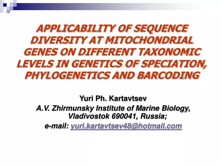
APPLICABILITY OF SEQUENCE DIVERSITY AT MITOCHONDRIAL GENES ON DIFFERENT TAXONOMIC LEVELS IN GENETICS OF SPECIATION, PHYLOGENETICS AND BARCODING. Yuri Ph. Kartavtsev A.V. Zhirmunsky Institute of Marine Biology, Vladivostok 690041, Russia ; e - mail : yuri.kartavtsev 48@ hotmail . com.

E N D
APPLICABILITY OF SEQUENCE DIVERSITY AT MITOCHONDRIAL GENES ON DIFFERENT TAXONOMIC LEVELS IN GENETICS OF SPECIATION, PHYLOGENETICS AND BARCODING Yuri Ph. Kartavtsev A.V. Zhirmunsky Institute of Marine Biology, Vladivostok 690041, Russia; e-mail: yuri.kartavtsev48@hotmail.com
Teacher: Academician, prof. Yuri P. Altukhov, 1992-2006 director, N.Vavilov Institute of General Genetics, Moscow (Russia)
MAIN GOALS • CBOL & Fish-BOL • SPECIES IDENTIFICATION • SPECIES DEFINITIONAND SPECIES ORIGIN:PROBLEMS, RESTRICTIONS. GENETIC VIEW.
THE INTERNATIONAL CBOL PROJECT • The CBOL is main global initiative. The Fish-BOL, its part, has over 5400 species barcoded by Co-1 from more than 30,000 specimens what makes it unique. P. Hebert and B. Hanner are preparing a $150M grant application for Genome Canada only for 2008. Othernations’ funds in CBOL are also big in some countries and unions: USA, EU. • B. Hanner suggests a recent Fish-BOL paper on Canadian freshwater fishes for your interest, as well as a new paper in press that demonstrates barcoding can identify cases of market substitution in North American seafood. These might be relevant for our meeting and ensuing discussions! • In this year there will be held third world-wide internationalconference (Sept. 2008 Chindao, Peoples Republic of China) and many regional meeting like us were performed.
THE INTERNATIONAL FISH-BOL PROJECT Cochairmen: P. Hebert &B. Ward
Registration and Barcoding Utilities(BolD; www.boldsystems.org) (1)
Registration and Barcoding Utilities(BolD; www.boldsystems.org) (2)
Registration and Barcoding Utilities(BolD; www.boldsystems.org) (3)
Chair:Masaki Miya Vice Chair:Shunping He Members: Nina Bogutskaya Seinen Chow Shunping He Yuri Kartavtsev Keiichi Matsuura Masaki Miya Mutsumi Nishida Ekaterina Vasilieva North East Asian Regional Working Group
Some Objects A B Fig. 1.Halibut-like flatfish,Hypoglossus elasodon(A) andobscure flatfish, Pseudopleuronectes obcurus (В).
INTRODUCTION • Mitochondrion DNA (mtDNA) is a ring moleculeof 16-18 kilo-base pairs (kbp) in length. As literature data show, mtDNA of all fisheshas similar organization (Lee et al., 2001; Kim et al., 2004; Kim et al., 2005; Nagase et al., 2005; Nohara et al., 2005) andsmall differencesamong all vertebrate animals, including men (Anderson et al., 1981; Bibb et al., 1981; Wallace, 1992; Kogelnik et al., 2005). • The complete content of whole mitochondrial genome (mitogenome) includes: control region (CRorD loop), where the siteof initiation of replication and promoters are located, big (16S) and small (12S) rRNA subunits, 22 tRNAand 13polypeptide genes. • Usually in phylogenetic research single gene sequences are usedfor both mtDNA and nuclear genome. However, recently more and more frequent are become complete mitogenome usage. Japanese scientists are leading here for water realm organisms. • Most popular in phylogenetics are sequences ofcytochrome b(Cyt-b) and cytochromeoxidase 1 (Cо-1) genes, which used for taxa comparison at the species - familylevel (Johns, Avise, 1998; Hebert et al., 2004; Kartavtsev, Lee, 2006). Many sequences that bringing the phylogenetic signal obtainedfor different taxaat gene 16S rRNA as well. • Sequences ofseparate genes can dive different phylogeneticsignal because of differences in substitution rates. This is also true for different sections of genes.Also, under comparison of higher taxa there may be effects of homoplasy. When numerous taxa available there are problemsof insufficient information capacity of sequences to cover big species diversity and representative taxa representation is quite important (Hilish et al., 1996). Nevertheless, for the species identification, excluding rare cases, fine results are availableeven with the usage of short sequences, like Со-1,with 650bp.
Applicability of Different DNA Typesin Phylogenetics and Taxonomy Spacers [ITS-1, 2] mtDNA nDNA, rDNA SpeciesGenusFamilyOrderClassPhylum Most substantiated statistically results Statistically significant results
p-DISTANCES IN GROUPS OF COMPARISON,Catfish Fig. 1.Resulting graph of mean p-distance values at four levels of differentiation in the catfish species (Siluriformes) for Cyt-b gene. Groups: 1. Intraspecies, among individuals of the same species; 2. Intragenus, among species of the same genera; 3. Intrafamily, among genera of the same family; 4. Intraorder, families of the order Pleuronectiformes. There are statistically significant variation. SE: a standard error of mean; F = 124.74, d.f. = 3; 29, p < 0.0001 (Kartavtsev et al., 2007a, Gene).
p-DISTANCES IN GROUPS OF COMPARISON,flatfish Fig. 2. Resulting graph of one factor ANOVA and mean p-distance values at four levels of differentiation in the flatfish species (Pleuronectiformes) for Cyt-b gene. Groups: 1. Intraspecies, among individuals of the same species; 2. Intragenus, among species of the same genera; 3. Intrafamily, among genera of the same family; 4. Intraorder, families of the order Pleuronectiformes. Statistically significant variation are shown on top of the graph. SE: a standard error of mean (Kartavtsev et al., 2007b, Marine Biol.).
p-DISTANCES IN GROUPS OF COMPARISON,turtles Fig. 3.Resulting graph of ANOVA and mean p-distance values at four levels of differentiation in turtle species (Testudines) for Cyt-b gene. Groups: 1. Intraspecies, among individuals of the same species; 2. Intragenus, among species of the same genera; 3. Intrafamily, among genera of the same family; 4. Intraorder, families of the same order. Variation among four groups is statistically significant: F = 61.87, d.f. = 3; 152, p < 0.000001 (Jungetal., 2006). р-Distances: (1) 2.33±0.03%, (2) 3.34±0.48%, (3) 6.41±0.11% и (4) 11.92±0.37% (Mean ± SE).
p-DISTANCES IN GROUPS OF COMPARISON,Perciformes Fig. 3. Resulting graph of one factor ANOVA and mean p-distance values at four levels of differentiation in fish species (Perciformes) for Co-1 gene sequence data. Comparison groups: 1. Intraspecies, among individuals of the same species; 2. Intragenus, among species of the same genera; 3. Intrafamily, among genera of the same family; 4. Intraorder, families of the order Perciformes. Variation is statistically significant. Bars are confidence intervals for mean (95%).
p-DISTANCES IN GROUPS OF COMPARISON,Review Fig. 4.Categorized plot of distribution of weighted mean p-distances among four groups of comparison at Cyt-bandCo-1genes. Groups here: 1. Intra-species, among individuals of the same species; 2. Intra-sibling species, 3. Intra-genus, among species of the same genera; 4. Intra-family, among genera of the same family (Kartavtsev, Lee, 2006).
GENETIC SIMILARITY IN TAXA OF DIFFERENT RANK: MEAN FOR THE GROUPS Fig. 5. Genetic similarity in taxa of different rank based on protein markers: mean for the groups. 1.Subspecies, 2.Semispecies and sibling species, 3.Species, 4.Genera. Intraspecies genetic distances were measured for many groups of organisms (Lewontin, 1974, Nei, 1987, Altukhov, 1989). Mean genetic similarity on this level is near I = 0.95 (see details in Kartavtsev, 2005). mtDNA data were presented above. Thus, data available suggest that in general a phyletic evolution prevail in animal world, and so far, the Geographic speciation events (Type 1a) prevail in nature. Do data presented assume that speciation is alwaysfollows the Type 1a mode? I guess, no. Few examples below let to support this answer.
DISTANCE VS TAXA SPLITTING • Has punctuation an impact in species origin on molecular level? • Avise, Ayala, 1976; Kartavtsev et al., 1980; current – No. • Pegel et al., 2006 – Yes. rs = 0.22, p < 0.05 Number of Splittings Transformed p-distance Fig. 6. Plot of p-distance on number of splittings at Cyt-b sequence data for catfishes and flatfishes.
GENETIC DISTANCES AMONG SPECIES IN SEPARATE ANIMAL GENERA(After Avise, Aquadro, 1982) This plot illustrate a thought that different animal groups of the same rank are unequal in structural gene divergence; i.e. the rate of evolution differ either at genes or at morphology or both.
GENETIC DISTATNCES IN TAXA OF SALMON FISHES D 1 – Populations within species, 2 – Subspecies, 3 - Species This plot support a thought that in salmon even a very small structural gene change can create separate biological species.
EXAMPLES OF REGULATORY DIVERGENCE IN FISH TAXA Comparison of chars Table 2.1. COMPARISON OF ISOZYME ACTIVITY IN THREE WHITEFISH FORMS (COREGONIDAE) AND GRAYLING (THYMALLIDAE) LEVELS OF DIFFERENCES IN ACTIVITY LOCUS/ FORM Ratio, % Note. Total number of loci analyzed are: Whitefish – 22, Grayling – 23, “-” – Activity do not differ significantly, “+” Iterative activity difference, “++” – two-fold difference, “+++” – three-fold or greater difference
WHAT IS MAIN OUTCOME • Distance measure alone is not satisfactory descriptor. • Data on intraspecies diversity (heterozygosity) at structural genes are necessary. • Measures of regulatory genome changes should be necessary to describe transformative modes of speciation. • Other descriptors of genomic change are required (e.g. chromoseme number, NF, etc.).
3. SPECIES DEFINITIONAND SPECIES ORIGIN:PROBLEMS, RESTRICTIONS.GENETIC VIEW
WHAT SPECIES IS? Species is a biological unity which reproductively isolated from other unities and consisting from one to several more or less stable populations of sexually reproducing individuals that occupy certain area in nature (my definition). In principal points, this is the definition of BSC (Biological Species Concept). In one of the original BSC definitions “A species is a reproductive community of populations (reproductively isolated from others) that occupies a specific niche in nature” (Mayr, 1982, p. 273). We will accept BSC for further discussion, although will keep in mind that it is restricted mainly to bisexual organisms (Mayr, 1963, Timofeev-Resovsky et al., 1977, Templeton, 1998). • The Linnaean Species • The Biological Species Concept (BSC) (Mayr, 1942, 1963) • BSC Modification II (Mayr, 1982) • The Recognition Species Concept (Paterson, 1978, 1985) • The Cohesion Species Concept (Templeton, 1989) • Evolutionary Species Concept • Simpson (1961) Evolutionary Species Concept. • Wiley’s (1978) Evolutionary Species Concept. • The Ecological Species Concept (Van Vallen, 1976). • The Phylogenetic Species Concept (Crawcraft, 1983).
GENERAL GENETIC APPROACH: ADVANCES AND LIMITATIONS • The problem of biological species, and speciation are main focus of this report. These problems took researcher’s attention since establishing the biology as a science. Most popular now among biologist is the Synthetic Theory of Evolution (STE), which part is comprised by the Biological Species Concept (BSC). Origin and systematic description of STE concept was presented in fundamental books by Haldane (1932), Dobzhansky (1937, 1943, 1951), Huxley (1954), Mayr and co-workers (Mayr, 1942, Mayr, 1963). A popular in Russia summary of STE became a book by Timofeev-Resovsky with co-authors (1977). Good, constructive ideas in STE support were developed by Vorontsov (1980). • One of weak point in STE is absence as a rule a possibility to prove experimentally one of key criteria of BSC – i.e., reproductive isolation of the species in nature. There are a lot of other criticisms that were summarized for example by King (1993). Nowadays, the new controversy between BSC and Phylogenetic Species Concept arise (Avise, Wollenberg, 1997). The theory of speciation is also not well developed in STE. Exactly speaking, in a quantitative meaning there is no theory as real matter at all. • In should be outlined, nevertheless, that many directions of STE and genetics of speciation are developing. Thus, a diverse analysis performed to understand a genetic sense and conceptual basements of speciation (Fox, Morrow, 1981, Grant, 1984, King, 1992). The genetic basis for creation of a reproductive isolationwas subjected to the analysis too (Leslie, 1982, Templeton, 1981, Nei et al., 1983, Coyne, 1992). As well there were considered: a possibility of a sympatric speciation (Bush, 1975, Genermon, 1991), the role of saltations or revolutions in evolution (Altukhov, Rychkov, 1970, Carson, 1974, Altukhov, 1985, 1997) and the genetic differentiation during formation of living forms and taxa (Avise, 1975, Avise, Aquadro, 1982, Nevo, Cleve, 1978, Thorpe, 1982, Nei, 1975, 1987).What in general are the advances and limitations in contemporary genetic approach?
ADVANCES • 1. Data reduction up to genotypic codes (values) give us a possibility to use genetic theory in the analysis. • 2. It is possible to perform a comparative investigation of a variability among structural and regulatory elements of the genome and genetic divergence of taxa. • 3. Investigations on protein and nucleotide divergence of species from nature discovered a “Molecular clock”. • 4. A possibility of phylogenetic reconstruction occurred: 1) not by similarity, but by kinship and 2) by in time dating of a divergence.
LIMITATIONS • 1. Deduction is limited by genotypic descriptions and genetic theory. • 2. Analysis is connected with preliminary laborious experimental investigation (with its own limitations). • 3. Investigation of a species from nature is frequently limited by originality or rare repetition of an event (phenomenon). • 4. Genotypic effects of the marker loci on phenotype are weak. • 5. The theory is not sufficiently developed in some directions.
WHAT DATA ARE NECESSARY? • Data that support (reject) central dogma of Neodarwinism – Evolution can occurred the only on the base of genetic change. • Data on variability at different levels of biological organization in genetic terms (by loci quantitative genotypic values – AA, …) – single-dimensioned data tables (DT). • Data on genotypic values of an individual at the set of loci (genotype – AA Bb…) or whole gene sequence set – multi-dimensionalDT. • Complementary data: Morphology traits, data on abiotic variability etc. (at least as an expert estimate – grouping variables).
SCHEMATIC REPRESENTATION OF SPECIES DIVERGENCE AND ORIGIN(FromDobzhansky, 1955) Fig. 3.1.Dobzhansky’s (1955) scheme of in time divergence. А – Single species population. B – Initial phase of divergence (subspecies). C – Different species. C The keystone of STE (Synthetic Theory of Evolution) may be represented by Dobzhansky’s scheme (Fig. 3.1), in which the gene pool separation is a key to speciation. If one provides a fact that evolution is possible without genetic change in lineages, then the evolutionary genetic paradigm and STE in particular can be rejected. B A
FIG. 3.2. DIAGRAMMATIC REPRESENTATION OF BASIC MODES OF SPECIATION(From Bush, 1975) Fig. 3.1. Main Modes of SpeciationBush, 1975) The gene flow breaks are able to create Reproductive Isolating Barriers (RIB) or Reproductive Isolation Mechanisms (RIM), which in their turn lead to further origin of species; under different situation in nature, the different modes of speciation acted (Fig. 3.2). Neither, the scheme above, nor the paper itself (Bush, 1975), answer many fundamental questions of speciation. For instance, it is unclear, what mode is most frequent and is a gene flow the sole primary factor, that alter gene pools or there are others? In other words we have to conclude that there is no a theory of speciation in scientific meaning at all.
SPECIATION MODES (SM): POPULATION GENETIC VIEW • ABSENCE OF QUANTITATIVE THEORY OF SPECIATION (QTS) • We have mentioned in preceding section that the speciation theory in evolutionary genetics is absent in exact scientific meaning, which expects the ability to predict future by the theory. In this case this is to predict species origin, or at least discriminate among several speciation modes on the basis of some quantitative parameters or their empirical estimates. Attempts made in this direction (Avise, Wollenberg, 1997, Templeton, 1998) do not fit the above criteria. That is why we attempted to step in the discrimination of the speciation modes on the basis of main population genetic measurements available in literature, and that may be laid in the frame of a genetic speciation concept. • BASEMENT FOR THE QTS • As a basis for the set of evolutionary genetic concepts we used the descriptions made by Templeton (1981). As a result the classification scheme for 7 different modes of speciation was created (Fig. 3.3). This approach leads to quite simple experimental scheme that permits: (i) to arrange further investigation of speciation in different groups of organisms, and (ii) to derive analytical relations for each speciation mode (Fig. 3.4). The approach is based on a set theory but it is aknowledge-based approach.I believe, this approach is best for such complicated matter.
Fig. 3.3.SPECIATION MODES (SM): POPULATION GENETIC VIEW(Kartavtsev et al, 2002) DIVERGENCE SM D1. ADAPTIVE D2. CLINAL D3. HABITAT DESCRIPTORS: D – Genetic distance at structural genes: DT – in suggested parent taxa, DS – among conspecific demes, DD – among subspecies or sibling species; HD – Mean heterozygosity in suggested daughter population; Hp – Mean heterozygosity in suggested parent population; EP – Divergence in regulatory genes among suggested parent taxa; ED – Divergence in regulatory genes among suggested daughter taxa; TM+- Test for modification (positive); TM-- Test for modification (negative). RIB – Reproductive isolation Barriers. Necessary Conditions for Speciation D1. a) Erection of extrinsic Isolating barriers followed by gene flow break; b) Pleotropic origin of RIB (Reproductive Isolatiion Barriers) in long time D2. a) Selection on a cline with isolation by distance; b) Pleotropic origin of RIB D3. a) Selection over multiple habitats with no isolation by distance; b) RIB origin by disruptive selection at genes determined behavior Sufficient Conditions for Speciation Lack of efficient hybridi- zation in the zone of contact Lack of efficient hybridi- zation outside the zone of contact Lack of efficient hybridi- zation inside and outside the zone of contact 1. DT > DS1 (S) 2. ED = EP 3. HD = HP 4. TM- 1. DT > DS2 (S) 2. ED EP 3. HD = HP 4. TM- 1. DT = DS3 (S) 2. ED EP 3. HD =< HP 4. TM- Experimentally measurable features and possible descriptors for the model (theory), (S)
1 (S) {(DT > DS) (ED = EP) (HD = HP) TM-} (D1) 2 (S) {(DT = DS) (ED EP) (HD = HP) TM-} (D2) 3 (S) {(DT = DS) (ED EP) (HD <= HP) TM+} (D3) 4 (S) {(DT > DD) (ED EP) (HD < HP) TM-} (T1) 5 (S) {(DT = DD) (ED = EP) (HD < HP) TM-} (T2) 6 (S) {(DT > DD) (ED EP) (HD > HP) TM-} (T3) 7 (S) {(DT > DS) (ED EP) (HD < HP) TM-} (T4) Fig. 3.4. ANALITICAL DESCRIPTION OF SEVEN TYPES OF SPECIATION MODES Note. Descriptors are explained in previous figure.
THE QTSEMPIRICAL PROVING • Salmon (Kartavtsev, Mamontov, 1983, Kartavtsev et al., 1983), • Cypriniformes (Kartavtsevetal., 2002), • Turtles, flatfishes,catfishes (Jung et al., 2006, Kartavtsev et al., 2006, 2007).
SPECIES IDENTIFICATION AND PHYLOGENETICS Phylogenetics + Taxonomy Identification + Taxonomy
Fig. 3.5. Rooted consensus (50%) trees (A-B) showing phylogenetic interrelationships on the basis of Cyt-b sequence data for the analyzed flatfish species (Pleuronectiformes) and four out-group taxa. A – tree based on NJ clustering technique with bootstrap support shown in the nodes (n=1000), B – Bayesian tree; repetition frequencies for n=106 simulated generations are shown (%) in the nodes. The tree was built based on the TrN+I+G model and was rooted with the sequences of four out-group species: three are Perciformes and one is Cypriniformes. The scales in the left bottom corners indicate relative branch lengths.
Fig. 3.6. Consensus (50%) tree showing phylogenetic interrelationships on the basis of Co-1 sequence data for the analyzed flatfish species (Pleuronectiformes) and two outgroup taxa. Rooted Bayesian tree; repetition frequencies (probabilities) for n=106 simulated generations are shown in the nodes (%).The tree was built based on the TVM+I+G model and rooted with the sequences of two outgroup species, Perciformes. The scale in the left bottom corners indicate the relative branch lengths.
Fig. 3.7.Rooted consensus (50%) tree showing phylogenetic interrelationships on the basis of Cyt-b sequence data for the analyzed flatfish species (Pleuronectiformes) and three outgroup taxa. Bayesian tree; repetition frequencies for n=106 simulated generations are shown (%) in the nodes. The trees were built based on the TrN+I+G model, and rooted with the sequences of outgroup species – Perciformes. The scales in the left bottom corners indicate the relative branch lengths.(Kartavtsev et al., 2007, Marine Biol.).
Fig. 3.8. Consensus (50%) trees showing phylogenetic interrelationships on the basis of Co-1 sequence data for 7 analyzed perch-like fish species (Perciformes) and two outgroup sequences. Rooted Bayesian tree was build for sample purposes; posterior probabilities for n=106 simulated generations are shown in the nodes (%). The tree was built based on the HKY+G model. Two other numbers in the nodes show tree bootstrap support based on similar clustering for NJ and ML techniques; support scores are given in the order NJ/ML/BA. Outgroup are two sequences of a representative of Cypriniformes. The scale in the left bottom corner indicate the relative branch lengths.
Conclusions • Speciation mode must be specified with a set of descriptors not exclusively by distances • Both Co-1 and Cyt-b are generally good barcoding tools for species identification • For phylogenetic reconstructions we need to cover both taxa diversity and several genes’ sequence diversity
THANKS FOR ATTENTION! СПАСИБО ЗА ВНИМАНИЕ!