Download
1 / 17
170 likes | 390 Vues
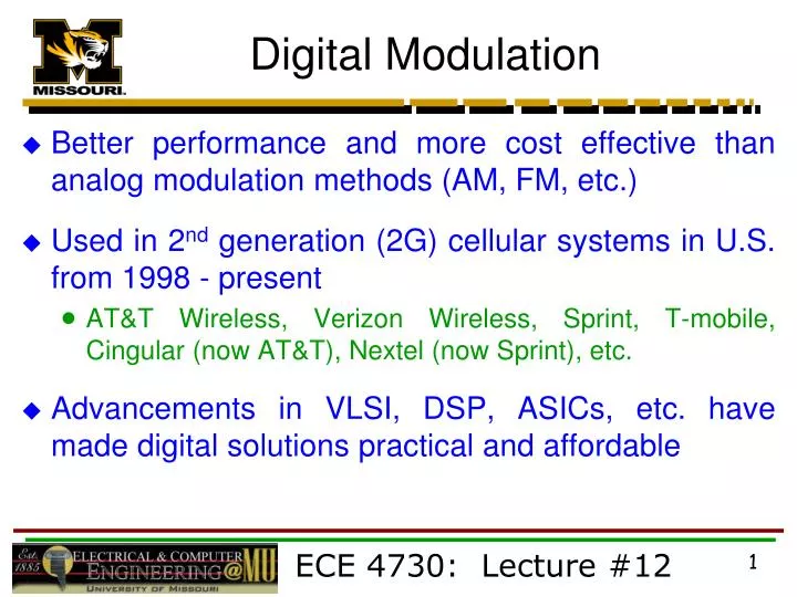
Digital Modulation. Better performance and more cost effective than analog modulation methods (AM, FM, etc.) Used in 2 nd generation (2G) cellular systems in U.S. from 1998 - present AT&T Wireless, Verizon Wireless, Sprint, T-mobile, Cingular (now AT&T), Nextel (now Sprint), etc.

E N D
Digital Modulation • Better performance and more cost effective than analog modulation methods (AM, FM, etc.) • Used in 2nd generation (2G) cellular systems in U.S. from 1998 - present • AT&T Wireless, Verizon Wireless, Sprint, T-mobile, Cingular (now AT&T), Nextel (now Sprint), etc. • Advancements in VLSI, DSP, ASICs, etc. have made digital solutions practical and affordable ECE 4730: Lecture #12
Digital Modulation • Performance advantages: 1) Resistant to noise, fading, & interference 2) Combine multiple information types (voice, data, & video) in single transmission channel 3) Improved security (e.g. encryption) deters phone cloning + eavesdropping 4) Error coding to detect/correct transmission errors 5) Signal conditioning to combat hostile MRC environment 6) Implement mod/dem functions using DSP software ECE 4730: Lecture #12
Digital Modulation Performance • Many types of digital modulation methods subtle differences • How to choose appropriate method?? • Performance factors to consider 1) Low Bit Error Rate (BER) at low SNR power efficiency 2) Resistance to interference (ACI & CCI) & fading 3) Occupies minimum amount of BW spectral efficiency 4) Easy and cheap to implement mobile unit 5) Efficient use of battery power mobile unit ECE 4730: Lecture #12
Digital Modulation Performance • Power Efficiency p • Ability of modulation technique to preserve quality of digital message at low power levels (low SNR) • Specified as Eb/No @ some BER (e.g. 10-5) where • Eb : energy/bit and No : noise energy/bit • Tradeoff between signal power vs. signal quality BER as Eb / No • **Note that this is NOT related to DC/RF efficiency of Tx power amplifier** ECE 4730: Lecture #12
Digital Modulation Performance • Bandwidth Efficiency B • Ability of modulation technique to accommodate data in a limited BW • Tradeoff between data rate (R) and occupied BW • BW as R • Symbol Period = Ts • Signal BW = Bs1 / Ts R ECE 4730: Lecture #12
PSD . . . f 1 / Ts = FNBW 0 0 0 1 0 0 1 1 Symbol Period = Ts Signal BW = Bs1 / Ts Digital Modulation Performance • For a digital signal : • Each pulse or “symbol” having mfinite states represents n = log2m bits/symbol e.g. m = 0 or 1 (2 states) n = 1 bit/symbol ECE 4730: Lecture #12
Digital Modulation Performance • Maximum BW efficiency Shannon’s Theorem C: channel capacity (bps) B : RF BW • Note that CB (expected) but also C S/N unexpected?? • Increase in signal power translates to increase in channel capacity!! • Large S/N easier to differentiate between multiple signal states (m) in one symbol n • is fundamental limit that cannot be achieved in practice typically only 4060% is realizable where ECE 4730: Lecture #12
Digital Modulation Performance • Fundamental tradeoff between pand B (in general) • If p then B (or vice versa) • Example: add error control bits to data stream and keep same data rate • Ts so Bs so B … but error bits will allow lower Eb / No for same BER so p • Is p vs. Btradeoff worth it?? • Use other factors to evaluate complexity, resistance to MRC impairments, etc. ECE 4730: Lecture #12
1 B’ 0.5 f fc B” B”’ Signal Bandwidth • Many definitions depending on application • All use Power Spectral Density (PSD) of modulated bandpass signal • FCC definition of occupied BW BW contains 99% of signal power B’ : half-power (3 dB) BW B” : null-to-null BW B’” : absolute BW range where PSD > 0 ECE 4730: Lecture #12
Tb 0 0 0 0 1 1 1 Tb 0 1 0 1 0 1 0 Line Coding • Different types of coding used for baseband digital signals • Choice depends on desired spectral properties • Unipolar 0 or V • Bipolar V or V • Non Return to Zero (NRZ) • Return to Zero (RZ) ECE 4730: Lecture #12
PSD Tb V 0 1 1 0 f . . . Rb = 1 / Tb Line Coding • Unipolar NRZ • Advantage : narrow spectral width • Disadvantage : large DC component data can’t be passed thru circuits that block DC (e.g. phone line!) • Disadvantage : no zero return hard to synchronize (decoding errors) ECE 4730: Lecture #12
PSD Tb V 0 . . . 1 0 1 f 2Rb = 2 / Tb Line Coding • Unipolar RZ • Disadvantage : wide spectral width • Advantage : smaller DC component • Advantage : better synchronization easier to decode ECE 4730: Lecture #12
PSD Tb +V 0 V V f 1 0 1 0 Rb 0.7Rb Line Coding • Manchester NRZ • Advantage : zero DC component • Advantage : zero crossing excellent synchronization • Moderate spectral width ECE 4730: Lecture #12
MRC Pulse Shaping • Rectangular pulses passed thru bandlimited channel (MRC) • Symbols smear into adjacent time slots • Inter-Symbol Interference (ISI) • Increases probability that symbol error will occur 0 1 0 1 0 1 0 1 ECE 4730: Lecture #12
Pulse Shaping • Spectral shaping of digital pulses done at baseband • Reduce ISI due to pulse smearing • Reduce spectral width of signal • Improve BW efficiency • Achieve better control of ACI! • Nyquist Criterion • Design overall response of system (Tx + MRC + Rx) so at every sampling instant in Rx (0/1 decision point) the response of all other symbols is zero • Leads to ideal “brick wall” filter in frequency domain ECE 4730: Lecture #12
Heff (f) f Pulse Shaping • Ideal Brick Wall Filter • In Time Domain -B +B ECE 4730: Lecture #12
Pulse Shaping • Ideal brick wall filter in frequency domain and unlimited time domain pulse response cannot be achieved in practice • Other filters can satisfy the Nyquist criterion • Raised Cosine (RC) Filter • Other pulse shaping filters can also be used that do NOT satisfy Nyquist criterion • Gaussian Filter ECE 4730: Lecture #12