Download
1 / 38
380 likes | 397 Vues
CHAPTER- 3 ERROR ANALYSIS T182,3.1-3.3. how to estimate uncertainties in our measurements, the sources of the uncertainties, and how to combine uncertainties in separate measurements to find the error in a result calculated from those measurements .

E N D
CHAPTER- 3 ERROR ANALYSIS T182,3.1-3.3
how to estimate uncertainties in our measurements, the sources of the uncertainties, and how to combine uncertainties in separate measurements to find the error in a result calculated from those measurements. • 3.1 INSTRUMENTAL AND STATISTICAL UNCERTAINTIES • Instrumental Uncertainties • the uncertainty in the measurement of quantity x which arise from a lack of perfect precision in the measuring instruments (including the observer) is called instrumental • These uncertainties are often independent of the actual value of the quantity being measured. • Instrumental uncertainties are determined by examining the instruments and considering the measuring procedure to estimate the reliability of the measurements. • In general, one should attempt to make readings to a fraction of the smallest scale division on the instrument. • The measurement is generally quoted to plus or minus one-half of the least count, and this number represents an estimate of the standard deviation of a single measurement. • for a Gaussian distribution, 68% probability that a random measurement will lie within 1 standard deviation of the mean • our objective in estimating errors to set a particular confidence level that a repeated measurement of the quantity will fall this close to the mean or closer. • Often we choose the standard deviation, the 68% confidence level, but other levels are used as well. • Digital instruments require special consideration. • Generally, manufacturers specify a tolerance; for example, the tolerance of a digital multimeter may be given as ± 1 %. • At any rate, the precision cannot be better than half the last digit on the display.
For example: if a student uses a resistor with a stated 1 % tolerance in an experiment, he can expect the stated uncertainty in the resistance to make a systematic contribution to all experiments with that resistor. • On the other hand, when he combines his results with those of the other students in the class, each of whom used a different resistor, the uncertainties in the individual resistances contribute in a statistical manner to the variation of the combined sample. • If it is possible to make repeated measurements, then an estimate of the standard deviation can be calculated from the spread of these measurements as discussed in Chapter 1. • The resulting estimate of the standard deviation corresponds to the expected uncertainty in a single measurement. • Statistical Uncertainties • If the measured quantity x represents the number of counts in a detector per unit time interval for a random process, then the uncertainties are called statistical uncertainties. • they arise from overall statistical fluctuations in the collections of finite numbers of counts over finite intervals of time. • For statistical fluctuations, we can estimate analytically the standard deviationforeach observation, without having to determine it experimentally. • If we were to make the same measurement repeatedly, we should find that the observed values were distributed about their mean in a Poisson distribution (as discussed in Section 2.2) instead of a Gaussian distribution.
The Poisson distribution and statistical uncertainties do not apply solely to experiment where counts are recorded in unit time intervals. • In any experiment in which data are grouped in bins according to some criterion to form a histogram or frequency plot, the number of events in each individual bin will obey Poisson statistics and fluctuate with statistical uncertainties. • One immediate advantage of the Poisson distribution is that the standard deviation is automatically determined: • = (3.1) • The relative uncertainty, the ratio of the standard deviation to the average rate, /= 1/, decreases as the number of counts received per interval increases. • Thus relative uncertainties are smaller when counting rates are higher. • The value for to be used in Equation (3.1) for determining the standard deviation is, of course, the value of the mean counting rate from the parent population, of which each measurement x is only an approximate sample. • In the limit of an infinite number of determinations, the average of all the measurements would very closely approximate the parent value, but often we cannot make more than one measurement of each value of x much less an infinite number. • Thus, we are forced to use x as an estimate of the standard deviation of a single measurement.
Example 3.1. • Consider an experiment in which we count gamma rays emitted by a strong radioactive source. • We cannot determine the counting rate instantaneously because no counts will be detected in an infinitesimal time interval. • But we can determine the number of counts x detected over a time interval t, and this should be representative of the average counting rate over that interval. • Assume that we have recorded 5212 counts in a I-s time interval. • The distribution of counts is random in time and follows the Poisson probability function, so our estimate of the standard deviation of the distribution is = 5212. • Thus, we should record our result for the number of counts x in the time interval tas 5212 ± 72 and the relative error is • There may also be instrumental uncertainties contributing to the overall uncertainties. • For example, we can determine the time intervals with only finite precision. • However, we may have some control over these uncertainties and can often organize our experiment so that the statistical errors are dominant. • Suppose that the major instrumental error in our example is the uncertainty t= 0.01 s in the time interval t = 1.00 s. • The relative uncertainty in the time interval is thus
This relative instrumental error in the time interval will produce a 1. % relative error in the number of counts x. • Because the instrumental uncertainty is comparable to the statistical uncertainty, it might be wise to attempt a more precise measurement of the interval or to increase its length. • If we increase the counting time interval from 1 s to 4 s, the number of counts x will increase by about a factor of 4 and the relative statistical error will therefore decrease by a factor of 2 to about 0.7%, whereas the relative instrumental uncertainty will decrease by a factor of 4 to 0.25%, as long as the instrumental uncertainty at remains constant at 0.01 s.
3.2 PROPAGATION OF ERRORS • want to determine a dependent variable x that is a function of one or more different measured variables. • how to propagate or carry over the uncertainties in the measured variables to determine the uncertainty in the dependent variable. • Example 3.2. • Suppose we wish to find the volume V of a box of length L, width W, and height H. • We can measure each of the three dimensions to be Lowidth Woand height H0 and combine these measurements to yield a value for the volume: • How do the uncertainties in the estimates Lo , Woand H0 , affect the resulting uncertainties in the final result Vo? • If we knew the actual errors, L = L - Loand so forth, in each dimension, we could obtain an estimate of the error in the final result Vo by expanding V about the point (Lo , Wo , Ho) in a Taylor series. • The first term in the Taylor expansion gives • from which we can find V = V - Vo. • The terms in parentheses are the partial derivatives of V, with respect to each of the dimensions, L, W, and H, evaluated at the point Lo , Wo , Ho.
.They are the proportionality constants between changes in V and infinitesimally small changes in the corresponding dimensions. • The partial derivative of V with respect to L, for example, is evaluated with the other variables W and H held fixed at the values Woand Hoas indicated by the subscript. • This approximation neglects higher-order terms in the Taylor expansion, which is equivalent to neglecting the fact that the partial derivatives are not constant over the ranges of L, W, and H given by their errors. • If the errors are large, we must include in this definition at least second partial derivatives and partial cross derivatives etcbut we shall omit these from the discussion that follows. • For our example of V = LWH, Equation (3.3) gives • which we could evaluate if we knew the uncertainties L, W, • and H.
Uncertainties • we may be able to estimate some characteristic of the error in each measured quantity, such as the standard deviation of the probability distribution of the measured qualities, • How can we combine the standard deviation of the individual measurements to estimate the uncertainty in the result?
Variance and Covariance • Combining Equations (3.8) and (3.9) we can express the variance x2 for x in terms of the variances u2, v2, . for the variables u, v, ... , which were actually measured: • The first two terms of Equation (3.10) can be expressed in terms of the variances u2, v2, given by Equation (1.8):
The first two terms in the equation are averages of squares of deviations weighted by the squares of the partial derivatives • may be considered to be the averages of the squares of the deviations in x produced by the uncertainties in u and in v, respectively. • In general, these terms dominate the uncertainties. • For any additional variables besides u and v in the determination of x, their contributions to the variance of x will have similar terms. • The third term is the average of the cross terms involving products of deviations in u and v weighted by the product of the partial derivatives. • If the fluctuations in the measured quantities u and v, . .. are uncorrelated, then, on the average, we should expect to find equal distributions of positive and negative values for this term, and we should expect the term to vanish in the limit of a large random selection of observations. • This is often a reasonable approximation and Equation (3.13) then reduces to with • similar terms for additional variables. • In general, we use Equation (3.14) for determining the effects of measuring uncertainties on the final result and neglect the covariant terms. • the covariant terms often make important contributions to the uncertainties in parameters determined by fitting curves to data by the least-squares method
3.3 SPECIFIC ERROR FORMULAS • The expressions of Equations (3.13) and (3.14) were derived for the general relationship of Equation (3.5) giving x as an arbitrary function of u and v, .... • In the following specific cases of functions f(u, v, ... ), the parameters a and b are defined as constants and u and v are variables. • Simple Sums and Differences
Example 3.3 • In an experiment to count particles emitted by a decaying radioactive source, we measure N1= 723 counts in a 15-s time interval at the beginning of the experiment and N2 = 19 counts in a 15-s time interval later in the experiment. • The events are random and obey Poisson statistics so that we know that the uncertainties in N1 and N2 are just their square roots. • Assume that we have made a very careful measurement of the background counting rate in the absence of the radioactive source and obtained a value B = 14.2 counts with negligible error for the same time interval t. • Because we have averaged over a long time period, the mean number of background counts in the 15-s interval is not an integral number. • For the first time interval, the corrected number of counts is: • x1 = N1- B = 723 - 14.2 = 708.8 counts • The uncertainty in x1 is given by: • x1= N1= 723 = 26.9 counts and the relative uncertainty is • For the second time interval, the corrected number of events is • x2 = N2- B = 19 - 14.2 = 4.8 counts • The uncertainty in x2is given by • x2= N2= 19 = 4.4 counts • and the relative uncertainty in x is:
Weighted Sums and Differences • If x is the weighted sum of u and v, • x = au + bv • the partial derivatives are simply the constants • and we obtain • Note the possibility that the variance x2 might vanish if the covariance uv2 v has the proper magnitude and sign. • This could happen in the unlikely event that the fluctuations were completely correlated so that each erroneous observation of u was exactly compensated for by a corresponding erroneous observation of v. • Example 3.4. • Suppose that, in the previous example, the background counts B were not averaged over a long time period but were simply measured for 15 s to give B = 14 with standard deviation B= 14 = 3.7 counts. • Then the uncertainty in xwould be given by • because the uncertainties in N and B are equal to their square roots. • For the first time interval, we would calculate • x1= (723 - 14) ± (723 + 14 ) = 709 ± 27.1 counts • and the relative uncertainty would be • For the second time interval, we would calculate • x2= (19 - 14) ± (19 + 14) = 5 ± 5.7 counts • and the relative uncertainty would be
Multiplication and Division • If x is the weighted product of u and v, • x = auv (3.21) • the partial derivatives of each variable are functions of the other variable, • and the variance of x becomes • which can be expressed more symmetrically as • Similarly, if x is obtained through division, • the relative variance for x is given by
Example 3.5. • The area of a triangle is equal to half the product of the base times the height • A = bh/2. • If the base and height have values b = 5.0 ± 0.1 cm and h = 10.0 ± 0.3 cm, the area is A = 25.0 cm2 and the relative uncertainty in the area is given by • Although the absolute uncertainty in the height is 3 times the absolute uncertainty in the base, the relative uncertainty is only times as large and its contribution to the variance of the area is only as large. • Example 3.6. • The area of a circle is proportional to the square of the radius A = r2. • If the radius is determined to be r = 10.0 ± 0.3 cm, the area is A = 100. cm2 with an uncertainty given by
Exponentials • If x is obtained by raising the natural base to a power proportional to u, • x = ae bu • the derivative of x with respect to u is • and the relative uncertainty becomes • If the constant that is raised to the power is not equal to e, the expression can • be rewritten as • where In indicates the natural logarithm. • Solving in the same manner as before we obtain
Logarithms • If x is obtained by taking the logarithm of u, • x = a In(bu) (3.38) • the derivative with respect to u is • Angle Functions • If x is determined as a function of u, such as • x = a cos(bu) (3.41) • The derivative of x with respect to u is • Note that uis the uncertainty in an angle and therefore must be expressed in radians. • These relations can be useful for making quick estimates of the uncertainty in a calculated quantity caused by the uncertainty in a measured variable. • For a simple product or quotient of the measured variable u with a constant, a 1 % error in u causes a 1 % error in x. • If u is raised to a power b, the resulting error in x becomes b% for a 1 % uncertainty in u. • Even if the complete expression for x involves other measured variables, x = f(u, v, ... ) and is considerably more complicated than these simple examples, it is often possible to use these relations to make approximate estimates of uncertainties.
3.4 APPLICATION OF ERROR EQUATIONS • Even for relatively simple calculations, such as those encountered in undergraduate laboratory experiments, blind application of the general error propagation expression [Equation (3.14)] can lead to very lengthy and discouraging equations, especially if the final results depend on several different measured quantities. • Often the error equations can be simplified by neglecting terms that make negligible contributions to the final uncertainty, but this requires a certain amount of practice. • Approximations • Students should practice making quick, approximate estimates of the various contributions to the uncertainty in the final result by considering separately the terms in Equation (3.14). • A convenient rule of thumb is to neglect terms that make final contributions that are less than 10% of the largest contribution. (Like all rules of this sort, one should be wary of special cases. • Several smaller contributions to the final uncertainty can sum to be as important as one larger uncertainty.)
Example 3.7. • Suppose that the area of a rectangle A = LW is to be determined from the following measurements of the lengths of two sides: • L=22.1±0.1 cm ; W= 7.3 ± 0.1 cm • The relative contribution of L to the error in L will be • and the corresponding contribution of wwill be • The contribution from Lis thus about one-third of that from w . • However, when the contributions are combined, we obtain • Thus, the effective contribution from Lis only about 6% of the effective contribution from wand could safely be neglected in this calculation.
Computer Calculation of Uncertainties Finding analytic forms for the partial derivatives is sometimes quite difficult. One should always break Equation (3.14) into separate components and not attempt to find one complete equation that incorporates all error terms. In fact, if the analysis is being done by computer, it may not even be necessary to find the derivatives explicitly. The computer can find numerically the variations in the dependent variable caused by variations in each independent, or measured, variable. Suppose that we have a particularly complicated equation, or set of equations, relating our final result x to the individually measured variables u, v, and so forth. Let us assume that the actual equations are programmed as a computer function CALCULATE, which returns the single variable x when called with arguments corresponding to the measured parameters x = CALCULATE(U, Y, W ... ) We shall further assume that correlations are small so that the covariances may be ignored. Then, to find the variations of x with the measured quantities u, v, and so forth, we can make successive calls to the function of the form DXU = CALCULATE(U + DU, Y, W, ... ) -x, DXY = CALCULATE(U, Y + DY, W,. ) - x, DXW = CALCULATE(U, Y, W + DW, ... ) - x, ETC. where DU, DV, DW, and so forth are the standard deviations u , v ,wand so on. The resulting contributions to the uncertainty in x are combined in quadrature as DX = SQRT(SQR(DXU) + SQR(DXY) + SQR(DXW) + ... ) Note that it would not be correct to incorporate all the variations into one equation such as DX = CALCULATE(U + DU, Y + DY, W + DW, ... ) - x because this would imply that the errors DU, DV, and so on were actually known quantities, rather than independent, estimated variations of the measured quantities,corresponding to estimates of the widths of the distributions of the measured variables.