Download
1 / 79
800 likes | 814 Vues
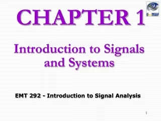
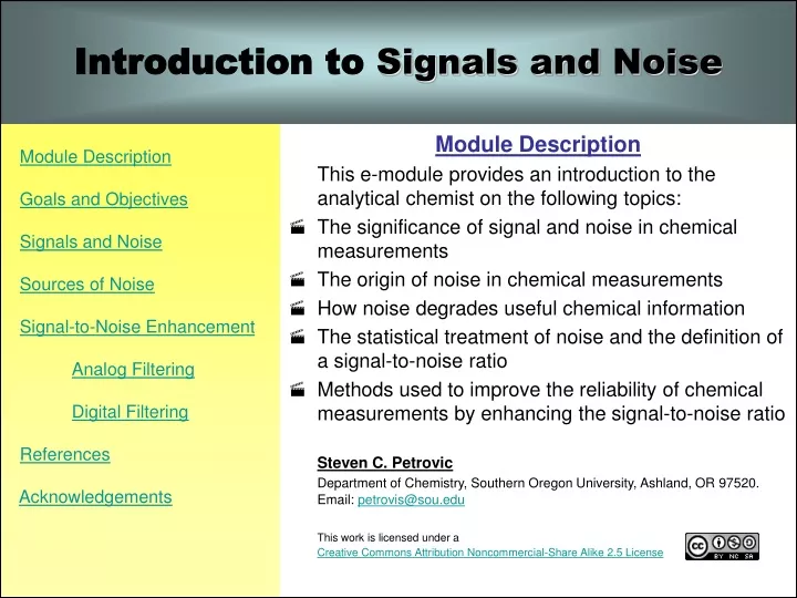
Introduction to Signals and Noise. Module Description Goals and Objectives Signals and Noise Sources of Noise Signal-to-Noise Enhancement Analog Filtering Digital Filtering References Acknowledgements. Module Description

E N D
Introduction to Signals and Noise Module Description Goals and Objectives Signals and Noise Sources of Noise Signal-to-Noise Enhancement Analog Filtering Digital Filtering References Acknowledgements Module Description This e-module provides an introduction to the analytical chemist on the following topics: • The significance of signal and noise in chemical measurements • The origin of noise in chemical measurements • How noise degrades useful chemical information • The statistical treatment of noise and the definition of a signal-to-noise ratio • Methods used to improve the reliability of chemical measurements by enhancing the signal-to-noise ratio Steven C. Petrovic Department of Chemistry, Southern Oregon University, Ashland, OR 97520. Email: petrovis@sou.edu This work is licensed under a Creative Commons Attribution Noncommercial-Share Alike 2.5 License
Introduction to Signals and Noise Module Description Goals and Objectives Signals and Noise Sources of Noise Signal-to-Noise Enhancement Analog Filtering Digital Filtering References Acknowledgements Goals and Objectives • Goal 1: This module will frame the roles of signal and noise in chemical measurements. • Objective 1: Define analytical signals and estimate signal parameters that correlate to analyte concentrations • Objective 2: Define noise, estimate the magnitude of noise, and investigate how the presence of noise interferes with the measurement of analytical signals • Objective 3: Define signal-to-noise ratio (S/N) as it relates to method performance and investigate how S/N is used to determine the detection limit of an analytical method • Goal 2: This module will describe how to improve the signal-to-noise ratio of analytical signals • Objective 1: Provide an introduction to the behavior of passive electronic circuits and show how they are used to improve the S/N of an analytical measurement • Objective 2: Provide an introduction to software-based methods and show how they are used to improve the S/N of an analytical measurement
Introduction to Signals and Noise Module Description Goals and Objectives Signals and Noise Sources of Noise Signal-to-Noise Enhancement Analog Filtering Digital Filtering References Acknowledgements NEXT Signals and Noise Defining Signal and Noise All analytical data sets contain two components: signal and noise Signal • This is the part of the data that contains information about the chemical species of interest (i.e. analyte). • Signals are often proportional to the analyte mass or analyte concentration • Beer-Lambert Law in spectroscopy where the absorbance, A, is proportional to concentration, C.
Introduction to Signals and Noise Module Description Goals and Objectives Signals and Noise Sources of Noise Signal-to-Noise Enhancement Analog Filtering Digital Filtering References Acknowledgements BACK NEXT Signals and Noise There are other significant relationships between signal and analyte concentration • The Nernst equation where a measured potential (E) is logarithmically related to the activity of an analyte (ax) • Competitive immunoassays (e.g. ELISA) where labeled (analyte spike) and unlabeled analyte molecules (unknown analyte) compete for antibody binding sites
Introduction to Signals and Noise Module Description Goals and Objectives Signals and Noise Sources of Noise Signal-to-Noise Enhancement Analog Filtering Digital Filtering References Acknowledgements BACK NEXT Signals and Noise Noise • This is the part of the data that contains extraneous information. • Noise originates from various sources in a analytical measurement system, such as: • Detectors • Photon Sources • Environmental Factors Therefore, characterizing the magnitude of the noise (N) is often a difficult task and may or may not be independent of signal strength (S). • A more detailed discussion on specific relationships between signal and noise may be obtained by clicking here and reading Section 3.
Introduction to Signals and Noise Module Description Goals and Objectives Signals and Noise Sources of Noise Signal-to-Noise Enhancement Analog Filtering Digital Filtering References Acknowledgements BACK NEXT Figure of Merit Why is Noise Unwanted? Noise degrades the accuracy and precision of a signal, and therefore our knowledge about how much analyte is present. Signal-to-Noise Ratio (S/N): A Figure of Merit The quality of a signal may be expressed by its signal-to-noise ratio
Introduction to Signals and Noise Module Description Goals and Objectives Signals and Noise Sources of Noise Signal-to-Noise Enhancement Analog Filtering Digital Filtering References Acknowledgements BACK NEXT Measuring Signals If the signal is at steady-state, as in the case of flame atomic absorption spectroscopy (FAAS), S is best estimated as the average signal magnitude, shown below by the solid line.
Introduction to Signals and Noise Module Description Goals and Objectives Signals and Noise Sources of Noise Signal-to-Noise Enhancement Analog Filtering Digital Filtering References Acknowledgements BACK NEXT Measuring Signals If the signal is transient, as in the case of chromatographic peaks, S is best estimated as the peak height or peak area. In the figure below, the peak height is measured from the midpoint of the baseline fluctuations (bottom horizontal line) to the top of the peak.
Introduction to Signals and Noise Module Description Goals and Objectives Signals and Noise Sources of Noise Signal-to-Noise Enhancement Analog Filtering Digital Filtering References Acknowledgements BACK NEXT Measuring Signals The peak area of a transient signal is the integrated response, which in this case has units of (µV*min). The peak area of this response is roughly equivalent to the area of the shaded triangle superimposed on the chromatographic peak.
Introduction to Signals and Noise Module Description Goals and Objectives Signals and Noise Sources of Noise Signal-to-Noise Enhancement Analog Filtering Digital Filtering References Acknowledgements BACK NEXT Quantifying Noise All data contains some level of uncertainty due to random fluctuations in the measurement process. We will focus on describing random fluctuations that may be described mathematically using a Gaussian distribution shown below. In this relationship: • y is the frequency that a value x will occur • µ is the population mean • σ is the standard deviation of the population
Introduction to Signals and Noise Module Description Goals and Objectives Signals and Noise Sources of Noise Signal-to-Noise Enhancement Analog Filtering Digital Filtering References Acknowledgements BACK NEXT Quantifying Noise Of course, there are such a myriad of samples and measurement methods that each case yields a unique distribution with a unique mean and standard deviation. In order to generally describe the Gaussian distribution, one must represent the Gaussian distribution in a standardized format. This can be done in two steps: • Mean-Centering subtracting the population mean from all the members of the data set so that µ = 0 • Normalization dividing each member of the data set by the distribution standard deviation so that σ = 1 The x-axis is now represented by a unitless quantity, z z = (x-µ)/σ
Introduction to Signals and Noise Module Description Goals and Objectives Signals and Noise Sources of Noise Signal-to-Noise Enhancement Analog Filtering Digital Filtering References Acknowledgements BACK NEXT Normal Error Curve If we look at a standardized Gaussian distribution – the so-called Normal Error Curve shown below – you can see that the probability of any one measurement being a member of this particular distribution increases as the magnitude of z increases.
Introduction to Signals and Noise Module Description Goals and Objectives Signals and Noise Sources of Noise Signal-to-Noise Enhancement Analog Filtering Digital Filtering References Acknowledgements BACK NEXT Normal Error Curve The area underneath the curve represented by “z” multiples of the standard deviation are shown in the table below:
Introduction to Signals and Noise Module Description Goals and Objectives Signals and Noise Sources of Noise Signal-to-Noise Enhancement Analog Filtering Digital Filtering References Acknowledgements BACK NEXT Calculating S/N Calculating the signal to noise ratio based on our brief discussion of Gaussian statistics can be achieved as follows: • Find a section of the data that contains a representative baseline. Notice that on the chart, the representative baseline does not contain any signal.
Introduction to Signals and Noise Module Description Goals and Objectives Signals and Noise Sources of Noise Signal-to-Noise Enhancement Analog Filtering Digital Filtering References Acknowledgements BACK NEXT Estimate peak-to-peak noise (VN) If the data is on a piece of paper, draw two lines that are parallel with the baseline and tangential to the edges of the baseline. See the example on the left side of the page. If the data is digitized (e.g. in a spreadsheet or text file), locate the maximum and minimum values in a representative section of the dataset that only represents the noise level.
Introduction to Signals and Noise Module Description Goals and Objectives Signals and Noise Sources of Noise Signal-to-Noise Enhancement Analog Filtering Digital Filtering References Acknowledgements BACK NEXT Estimate root mean square noise • Calculate the standard deviation (VRMS) of the noise. At the 99% confidence level: VN = ±2.58σ.Therefore: • Estimate the S/N. The signal is 16.0 µV.
Introduction to Signals and Noise Module Description Goals and Objectives Signals and Noise Sources of Noise Signal-to-Noise Enhancement Analog Filtering Digital Filtering References Acknowledgements BACK Estimating S/N First, calculate the standard deviation (VRMS) of the noise. At the 99% confidence level: VN= ±2.58σ.Therefore: Second, calculate the S/N. The signal is 16.0 µV.
Introduction to Signals and Noise Module Description Goals and Objectives Signals and Noise Sources of Noise Signal-to-Noise Enhancement Analog Filtering Digital Filtering References Acknowledgements NEXT Sources of Instrumental Noise • Johnson Noise Also called thermal noise, this source of noise results in random voltage fluctuations produced by the thermal agitation of electrons as they pass through resistive elements in the electronics of an instrument. The relationship between Johnson Noise and experimental parameters is as follows: VRMS:Root-mean-square noise voltage with a frequency bandwidth of Δf (in Hertz). k: Boltzmann’s constant (1.38 x 10⁻²³ J/K) T: Temperature (K) R: Resistance of resistive element (Ω) Reduction of Johnson Noise is accomplished most easily by: • Cooling the detector (reducing T) • Decreasing the frequency bandwidth of the signal (reducing Δf) • Actual measurements of Johnson Noise may be found by clicking here
Introduction to Signals and Noise Module Description Goals and Objectives Signals and Noise Sources of Noise Signal-to-Noise Enhancement Analog Filtering Digital Filtering References Acknowledgements BACK NEXT Sources of Instrumental Noise • Shot Noise This source of noise results in current fluctuations produced by electrons crossing a junction in a random fashion, which highlights the quantized nature of electron flow The relationship between Shot Noise and experimental parameters is as follows: iRMS:Root-mean-square current fluctuation (in Amperes) I: Average direct current (A) e: electronic charge (1.60 x 10⁻¹⁹ C) Δf: frequency bandwidth (Hz) Reduction of Shot Noise is accomplished most easily by: Decreasing the frequency bandwidth of the signal (reducing Δf) A good discussion of Shot Noise may be found by clicking here
Introduction to Signals and Noise Module Description Goals and Objectives Signals and Noise Sources of Noise Signal-to-Noise Enhancement Analog Filtering Digital Filtering References Acknowledgements BACK Sources of Instrumental Noise • Flicker Noise Flicker noise is also called 1/f noise because the magnitude of flicker noise is inversely proportional to frequency. The source of flicker noise is uncertain and it seems to be significant only at low frequencies (<100 Hz) A good summary of flicker noise (and Johnson noise) may be found by clicking here • Environmental Noise These are sources of noise that interfere with analytical measurements. Examples of such sources include: electrical power lines (e.g. 50 or 60 Hz line noise) electrical equipment (e.g. motors, fluorescent lights, etc.) RF sources (e.g. cell phones) environmental factors (drift in temperature, aging of electronic components)
Introduction to Signals and Noise Module Description Goals and Objectives Signals and Noise Sources of Noise Signal-to-Noise Enhancement Analog Filtering Digital Filtering References Acknowledgements NEXT Introduction to Signal-to-Noise Enhancement As the S/N of an analytical signal decreases, so does the accuracy and precision of that signal. The pair of plots below illustrate this point. The plot to the left contains three analyte peaks with a peak-to-peak noise level of 0.19 µV. The S/N for each peak is 52, 26, and 10 respectively. Increasing the peak-to-peak noise level ten-fold (1.9 µV) decreases the S/N of each peak by a factor of ten. (5.2, 2.6, 1.0 respectively)
Introduction to Signals and Noise Module Description Goals and Objectives Signals and Noise Sources of Noise Signal-to-Noise Enhancement Analog Filtering Digital Filtering References Acknowledgements BACK NEXT Introduction to Signal-to-Noise Enhancement Note that the signal at 2 minutes, with a S/N ratio of ~3, is at a level commonly known as the detection limit, which is defined as the magnitude at which the signal is statistically distinguishable from the noise. The signal at 3 minutes, which has a S/N equal to 1, is indistinguishable from the baseline noise. This comparison illustrates the need to reduce noise to a level at which chemical information is not compromised. A spreadsheet has been designed to illustrate the relationship between signal and noise. Click here to perform these exercises.
Introduction to Signals and Noise Module Description Goals and Objectives Signals and Noise Sources of Noise Signal-to-Noise Enhancement Analog Filtering Digital Filtering References Acknowledgements BACK NEXT Introduction to Signal-to-Noise Enhancement Can Noise be Reduced After the Data has been Recorded? In the examples below, the frequency of the signal is less than the frequency of the noise. In all cases, if the signal frequency and the noise frequency are not equal, then there should be at least one suitable approach to noise reduction.
Introduction to Signals and Noise Module Description Goals and Objectives Signals and Noise Sources of Noise Signal-to-Noise Enhancement Analog Filtering Digital Filtering References Acknowledgements BACK Overview of S-N Enhancement Techniques This module will describe two general categories of noise reduction techniques: • Analog Filtering (Hardware-Based) • Digital Filtering (Software-Based) Most of these S/N enhancement methods, whether analog or digital, are based on either: • Bandwidth Reduction (i.e. decreasing Δf). • Signal Averaging (i.e. decreasing Δf or averaging out random noise fluctuations) Bandwidth reduction is important --- Remember, if fsignal ≠ fnoise, we have a chance of isolating the signal from the noise. This results in an enhanced signal-to-noise ratio and more reliable information about the chemical sample of interest. We will see that there are limitations to how much bandwidth reduction can be applied before distorting the instrumental signal. Nevertheless, these can be effective approaches to improving the quality of the instrumental signal.
Introduction to Signals and Noise Module Description Goals and Objectives Signals and Noise Sources of Noise Signal-to-Noise Enhancement Analog Filtering Digital Filtering References Acknowledgements NEXT Analog Filtering Signals and noise are almost always expressed as electrical quantities. The electrical quantities you should be familiar with are: Voltage: Voltage is a measure of energy available when an electron moves from a point of higher potential to a point of lower potential. The SI Unit for voltage is the Volt (V). 1V = 1 Joule/Coulomb. Physicochemical phenomena that generate voltage include: • Chemical Reactions, such as those that take place in a battery • Electromagnetic Induction, such as moving a coil of wire through a magnetic field (i.e. an electric generator) • Photovoltaic Cells, which convert light energy into electrical work Current: Current is a measure of the amount of electronic charge flowing per unit time past a given point. The SI Unit for current is the Ampere (A). 1A = 1 Coulomb/second. Types of current include • Direct Current (DC): Charges are flowing in the same direction. • Here’s an applet that demonstrates the production of pulsed DC: http://micro.magnet.fsu.edu/electromag/java/generator/dc.html • Alternating Current (AC): Charges change direction periodically. • Here’s an applet that demonstrates the production of AC: http://micro.magnet.fsu.edu/electromag/java/generator/ac.html
Introduction to Signals and Noise Module Description Goals and Objectives Signals and Noise Sources of Noise Signal-to-Noise Enhancement Analog Filtering Digital Filtering References Acknowledgements BACK NEXT Analog Filtering - Ohm’s Law In 1827, Georg Ohm published his work Die galvanische Kette mathematisch bearbeitet, indicating that the current flowing through a conductor is proportional to the voltage across the conductor. All conductors of electricity obey Ohm’s Law, which is mathematically expressed as: V = Voltage across the conductor (in Volts, V) I = Current through the conductor (in Amperes, A) R = Resistance of the conductor (in Ohms, Ω) Simple applets to test out Ohm’s Law: http://micro.magnet.fsu.edu/electromag/java/ohmslaw/ http://phet.colorado.edu/simulations/veqir/VeqIRColored.swf http://www.walter-fendt.de/ph14e/ohmslaw.htm
Introduction to Signals and Noise Module Description Goals and Objectives Signals and Noise Sources of Noise Signal-to-Noise Enhancement Analog Filtering Digital Filtering References Acknowledgements BACK NEXT Passive Electronic Components Resistor • A resistor is a component that resists electron flow. • The unit of resistance is called an ohm (Ω). 1Ω = 1V/A • In an electronic circuit schematic, a resistor is represented by: Capacitor • A capacitor is an electronic component that stores charge • It consists of two conductive plates separated by an insulating medium • The unit of capacitance is called a farad (F). 1F = 1C/V • In an electronic circuit schematic, a capacitor is represented by: A simple applet used to illustrate the principle of resistance http://micro.magnet.fsu.edu/electromag/java/filamentresistance/index.html Simple applets used to illustrate the principle of capacitance http://micro.magnet.fsu.edu/electromag/java/capacitance/index.html http://micro.magnet.fsu.edu/electromag/java/capacitor/
Introduction to Signals and Noise Module Description Goals and Objectives Signals and Noise Sources of Noise Signal-to-Noise Enhancement Analog Filtering Digital Filtering References Acknowledgements BACK NEXT Passive Electronic Circuits Remember that signal-to-noise ratios can be enhanced if the signal frequency is different than the noise frequency. You will be introduced to these frequency-dependent analog filters at the end of this section. For now, let’s start very simply… Resistor Fundamentals The simplest circuit involving a resistor and a voltage source is shown below. The dotted lines are just there to represent where a high-quality voltmeter would be connected if we wished to measure the voltage across the resistor. Calculating the current flowing through this resistor requires the use of Ohm’s Law. Circuit #1 According to Ohm’s Law • V = 1.0 Volt • R = 20 Ohms
Introduction to Signals and Noise Module Description Goals and Objectives Signals and Noise Sources of Noise Signal-to-Noise Enhancement Analog Filtering Digital Filtering References Acknowledgements BACK NEXT Passive Electronic Circuits Resistors in Series Practically speaking, we are not limited to a single resistor. Circuit #1 could also be represented by Circuit #2 below: • Resistors placed in a “head-to-tail” configuration are in series. • The total resistance is the sum of all the individual resistances • Putting resistors together in series gives a larger total resistance
Introduction to Signals and Noise Module Description Goals and Objectives Signals and Noise Sources of Noise Signal-to-Noise Enhancement Analog Filtering Digital Filtering References Acknowledgements BACK NEXT Passive Electronic Circuits Resistors in Parallel Resistors placed in a “side-to-side” configuration are in parallel. The total resistance is the reciprocal of the sum of each reciprocal resistance. So for a pair of resistors as shown in Circuit #3 above: Applying this to Circuit #3: Putting resistors together in parallel always gives a smaller total resistance. Note that Circuit #3 has the same current as Circuits #1 and #2.
Introduction to Signals and Noise Module Description Goals and Objectives Signals and Noise Sources of Noise Signal-to-Noise Enhancement Analog Filtering Digital Filtering References Acknowledgements BACK NEXT Passive Electronic Circuits Voltage Divider Sometimes, the output of an instrument is too large for a readout device. One circuit used to reduce a voltage is a voltage divider Note that: • A representation for a voltmeter has been added to the schematic • The voltage is only being accessed across one of the two resistors
Introduction to Signals and Noise Module Description Goals and Objectives Signals and Noise Sources of Noise Signal-to-Noise Enhancement Analog Filtering Digital Filtering References Acknowledgements BACK NEXT Passive Electronic Circuits Voltage Divider (Page 2) Assuming that the meter resistance is much larger than R2 (i.e. no loading error occurs), then according to Ohm’s Law Vin = I(R1 + R2) For a discussion of loading errors, click here. Passive Electronic Circuits Voltage Divider (Page 2) Assuming that the meter resistance is much larger than R2 (i.e. no loading error occurs), then according to Ohm’s Law Vin = I(R1 + R2) For a discussion of loading errors, click here.
Introduction to Signals and Noise Module Description Goals and Objectives Signals and Noise Sources of Noise Signal-to-Noise Enhancement Analog Filtering Digital Filtering References Acknowledgements BACK NEXT Passive Electronic Circuits Voltage Divider (Page 3) If the readout device (i.e. a meter) is placed across R2, than the voltage read by the meter is Or in other words, the divider output equals the instrument output multiplied by R2 over the total resistance
Introduction to Signals and Noise Module Description Goals and Objectives Signals and Noise Sources of Noise Signal-to-Noise Enhancement Analog Filtering Digital Filtering References Acknowledgements BACK NEXT Passive Electronic Circuits Voltage Divider (Page 4) In this case, the divider output is:
Introduction to Signals and Noise Module Description Goals and Objectives Signals and Noise Sources of Noise Signal-to-Noise Enhancement Analog Filtering Digital Filtering References Acknowledgements BACK NEXT Passive Electronic Circuits RC Voltage Dividers (Analog Filters) Although voltage dividers are extremely useful, they are unable to selectively filter signal voltages from noise voltages. That is: Voltage dividers are frequency independent. However, the impedance of a capacitor is frequency dependent, as shown by the following equation: • XC is the impedance of the capacitor (impedance is the generalized form of resistance that applies to AC signals) • f is the frequency of the voltage source in Hertz • C is the capacitance in Farads As the frequency increases, the impedance of a capacitor decreases!
Introduction to Signals and Noise Module Description Goals and Objectives Signals and Noise Sources of Noise Signal-to-Noise Enhancement Analog Filtering Digital Filtering References Acknowledgements BACK NEXT Passive Electronic Circuits Low-Pass Filters • Used when the signal frequency < noise frequency • The relationship between Vin and Vout is analogous to a frequency independent voltage divider • The desired filter output is obtained across the frequency dependent component (capacitor)
Introduction to Signals and Noise Module Description Goals and Objectives Signals and Noise Sources of Noise Signal-to-Noise Enhancement Analog Filtering Digital Filtering References Acknowledgements BACK NEXT Passive Electronic Circuits High-Pass Filters • Used when the signal frequency > noise frequency • The relationship between Vin and Vout is analogous to a frequency independent voltage divider • The desired filter output is obtained across the frequency independent component (resistor)
Introduction to Signals and Noise Module Description Goals and Objectives Signals and Noise Sources of Noise Signal-to-Noise Enhancement Analog Filtering Digital Filtering References Acknowledgements BACK NEXT Decibel Scale Expressing Signal Attenuation of RC filters • Because an ideal analog filter would not attenuate the signal but only the noise, the decibel scale is used to express the degree of electrical attenuation (or gain) attributable to an electronic device, such as a RC filter. • A decibel is defined as: dB = 20 log (Vout/Vin) • So 0 dB represents no signal attenuation, and -20 dB represents an order of magnitude decrease in the RC filter output compared with the input. • Remember that S/N enhancement is possible if the frequency of the signal and the noise are different. We can express the attenuation of the RC filter response as a function of frequency using a Bode plot. • Bode plots are log-log plots: decibels are a logarithmic quantity and frequency is plotted on a logarithmic scale. They are quite frequently used to illustrate the frequency response of electronic circuits.
Introduction to Signals and Noise Module Description Goals and Objectives Signals and Noise Sources of Noise Signal-to-Noise Enhancement Analog Filtering Digital Filtering References Acknowledgements BACK NEXT Bode Plots • Below is a Bode plot of the low-pass RC filter frequency response shown a few slides back. Notice that low frequencies are unattenuated, but attenuation increases with higher frequencies.
Introduction to Signals and Noise Module Description Goals and Objectives Signals and Noise Sources of Noise Signal-to-Noise Enhancement Analog Filtering Digital Filtering References Acknowledgements BACK NEXT Bode Plots • Every Bode plot has two straight lines: the relatively flat response where little attenuation occurs and a linear response of -20 dB/decade at higher frequencies. The intersection point of these two lines coincides with the rounded section of the plot. This is the cutoff frequency, fo, of the RC filter, which is expressed by the following relationship: fo = 1/(2πRC) The cutoff frequency, which is 1592 Hz for this particular circuit, corresponds to a 3 dB attenuation, and can be used as a figure-of-merit for the response of the filter.
Introduction to Signals and Noise Module Description Goals and Objectives Signals and Noise Sources of Noise Signal-to-Noise Enhancement Analog Filtering Digital Filtering References Acknowledgements BACK NEXT Bode Plots • Below is a Bode plot of the high-pass RC filter frequency response a few slides back. Note that because the same resistor and capacitor was used, the cutoff frequency has not changed. The filter output is simply accessed across the resistor instead of the capacitor.
Introduction to Signals and Noise Module Description Goals and Objectives Signals and Noise Sources of Noise Signal-to-Noise Enhancement Analog Filtering Digital Filtering References Acknowledgements BACK Passive Electronic Circuits Analog Filter Demo A lecture demonstration of how an RC filter isolates noise from signal can be obtained as a MS Word document by clicking here or as a web page by clicking here. Bode Plot Exercise An exercise on interpreting the frequency response of RC filters using a Bode plot can be accessed by clicking here. Analog Filter Exercises A couple of exercises have been included to reinforce your understanding about the design and application of analog filters. • Click here to access Exercise #1 • Click here to access Exercise #2
Introduction to Signals and Noise Module Description Goals and Objectives Signals and Noise Sources of Noise Signal-to-Noise Enhancement Analog Filtering Digital Filtering References Acknowledgements NEXT Digital Filtering What is a digital filter? A digital filter is a noise reduction technique that is software-based. It is an approach that was popularized once personal computers became widely available. Digitally-based signal-to-noise enhancement techniques described in this e-module include: • Ensemble Averaging • Boxcar Averaging • Moving Average (Weighted & Unweighted)
Introduction to Signals and Noise Module Description Goals and Objectives Signals and Noise Sources of Noise Signal-to-Noise Enhancement Analog Filtering Digital Filtering References Acknowledgements BACK NEXT Digital Filtering Ensemble Averaging Ensemble averaging is a data acquisition method that the enhances the signal-to-noise of an analytical signal through repetitive scanning. Ensemble averaging can be done in real time, which is extremely useful for analytical methods such as: • Nuclear Magnetic Resonance Spectroscopy (NMR) • Fourier Transform Infrared Spectroscopy (FTIR) Ensemble averaging also works well with multiple datasets once data acquisition is complete. In either case, this method of S/N enhancement requires that: • The analyte signal must be stable • The source of noise is random
Introduction to Signals and Noise Module Description Goals and Objectives Signals and Noise Sources of Noise Signal-to-Noise Enhancement Analog Filtering Digital Filtering References Acknowledgements BACK NEXT Digital Filtering How Ensemble Averaging Works • Repeated experiments (scans) are performed on the chemical system in question. The scans are averaged either in real-time or after the data acquisition is complete. A visualization of this process is shown below for five spectra of 8.8 µg/mL 1,1’-ferrocenedimethanol in water.
Introduction to Signals and Noise Module Description Goals and Objectives Signals and Noise Sources of Noise Signal-to-Noise Enhancement Analog Filtering Digital Filtering References Acknowledgements BACK NEXT Digital Filtering Pros of Ensemble Averaging • Ensemble averaging filters out random noise, regardless of the noise frequency • Ensemble averaging is effective, even if the original signal has a S/N<1 • Ensemble averaging is straightforward to implement • Improvement in S/N is proportional to: Cons of Ensemble Averaging • Requirement of a stable signal • Ensemble averaging will not work if noise is not random (e.g. 60 Hz electrical noise)
Introduction to Signals and Noise Module Description Goals and Objectives Signals and Noise Sources of Noise Signal-to-Noise Enhancement Analog Filtering Digital Filtering References Acknowledgements BACK NEXT Digital Filtering Example of Ensemble Averaging These simulated 5-µV gaussian signals illustrate S/N improvement of ensemble averaging. The bottom dataset represents a S/N of 2 (single dataset), the middle dataset represents a S/N of 8 (average of 16 datasets), and the top dataset represents a S/N of 20 (average of 100 datasets). Click here to work on an ensemble averaging exercise.
Introduction to Signals and Noise Module Description Goals and Objectives Signals and Noise Sources of Noise Signal-to-Noise Enhancement Analog Filtering Digital Filtering References Acknowledgements BACK NEXT Digital Filtering Boxcar Averaging Boxcar averaging is a data treatment method that the enhances the signal-to-noise of an analytical signal by replacing a group of consecutive data points with its average. This treatment, which is called smoothing, filters out rapidly changing signals by averaging over a relatively long time but has a negligible effect on slowly changing signals. Therefore, boxcar averaging mimics a software-based low-pass filter. Boxcar averaging can be done both in real time and after data acquisition is complete. How Boxcar Averaging Works: During Data Acquisition: • The signal is sampled several times. Theoretically, any number of points may be used. • The samples are summed together and an average is calculated. • The average signal (dependent variable) is stored in the smoothed data set as the y-coordinate, and the average value of the independent variable (e.g. time, wavelength) is used as the x-coordinate.
Introduction to Signals and Noise Module Description Goals and Objectives Signals and Noise Sources of Noise Signal-to-Noise Enhancement Analog Filtering Digital Filtering References Acknowledgements BACK NEXT Digital Filtering How Boxcar Averaging Works: After Data Acquisition (see figure below): • Sum the data points within the boxcar • Divide by the number of points in the boxcar • Plot the average y-value at the central x-value of the boxcar • Repeat with Boxcar 2, etc until the last full boxcar is smoothed
Introduction to Signals and Noise Module Description Goals and Objectives Signals and Noise Sources of Noise Signal-to-Noise Enhancement Analog Filtering Digital Filtering References Acknowledgements BACK NEXT Digital Filtering Main Points about Boxcar Averaging: • Boxcar averaging is equivalent to software-based low-pass filtering. • Boxcar averaging is straightforward to implement. • Improvement in S/N is proportional to: • (N-1) points are lost from each boxcar in the smoothed data set, where N is the boxcar length. The data density of the smoothed data set will be reduced by (N-1)/N • Significant loss of information can occur if the length of the boxcar is comparable to the data acquisition rate. It is best to implement boxcar averaging with a sufficient data acquisition rate.