Download
1 / 36
360 likes | 375 Vues
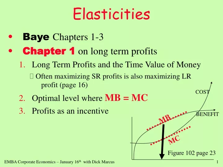
Elasticities. Baye Chapters 1-3 Chapter 1 on long term profits Long Term Profits and the Time Value of Money Often maximizing SR profits is also maximizing LR profit (page 16) Optimal level where MB = MC Profits as an incentive. COST. BENEFIT. MB. MC. Figure 102 page 23.

E N D
Elasticities • Baye Chapters 1-3 • Chapter 1 on long term profits • Long Term Profits and the Time Value of Money Often maximizing SR profits is also maximizing LR profit (page 16) • Optimal level where MB = MC • Profits as an incentive COST BENEFIT MB MC Figure 102 page 23
The Role of Profits • Economic Profitis the difference between revenues and total economic cost (including the economic or opportunity cost of owner supplied resources such as time and capital). • We’d expect high profit areas to attract investment • We’d expect low profit areas to lose investment • Shouldn’t then all industries earn the same profit eventually?
Profit Varies Theories on Why Across Industries • RISK-BEARING THEORY • TEMPORARY DISQUILIBRIUM THEORY OF PROFIT • MONOPOLY THEORY OF PROFIT • INNOVATION THEORY OF PROFIT • MANAGERIAL EFFICIENCY THEORY OF PROFIT
Five Forces of Competitive Advantage The forces that determine competitive advantage are: • Substitutes (threat of substitutes can be offset by brands and special functions served by the product). • Potential Entrants (threat of entrants can be reduced by high fixed costs, scale economies, restriction of access to distribution channels, or product differentiation). • Buyer Power (threat of concentration of buyers). • Input Supplier Power (threats from concentrated suppliers of key inputs affect profitability). • Intensity of Rivalry (market concentration, price competition tactics, exit barriers, amount of fixed costs, and industry growth rates impact profitability).
Figure 1.1 on Page 8 Potential Entry Entry Costs Speed of Adjustment Sunk Costs Network Effects Reputation Switching Costs Government Constraints Substitutes & Complements Price/Value of surrogates Branded vs. generic Sustainable industry profitability Intensity of rivalry Industrial concentration Pricing tactics Degree of Differentiation Switching costs Timing of decisions Information Buyer power Buyer concentration Price/Value of substitutes Customer Switching Costs Input Supplier power Supplier Concentration Supply Switching Costs Relationship-specific investments Government restraints
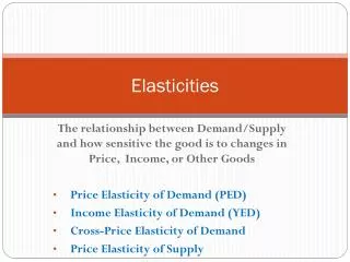
Chapter 2: Demand & Supply • Foundations class looked at individual and market demand as well as firm and market supply functions. • Consumer Surplus – area above price and below demand. (see Fig 2-5, page 45) • Producer Surplus – area below price and above supply (se Fig 2-9, page 51) • We also examined equilibrium, shifts in demand or supply called Comparative Statics, as well as price ceilings and floors. supply CS PS demand
Elasticities Baye: Chapter 3 – Quantitative Demand Analysis • Chapters 1 & 2 review, demand, supply & equilibrium we discussed in Foundations. • Elasticity is measure of responsiveness or sensitivity • Beware of using Slopes Slopes change with a mere change in the units of measure price price per per bu. bu bushels tons
Price Elasticity • Price elasticities are often given as the absolute value of their price elasticity for historical reasons. We’ll let them be negative numbers • Elasticity of Demand = eP ≡ EQ,P≡EP ≡ (% change in Q) / (% change in P) • Ratios of percentages are not affected by units of measure. They are pure numbers. -30% / 10% = -3 • Price elasticities are also known as own-price elasticities or demand elasticities.
Price Elasticitya.k.a “Own Price Elasticity of Demand” • E P = % change in Q / % change in P • Shortcut notation:E P = Q* / P* • A percentage change from 100 to 150 is 50% • A percentage change from 150 to 100 is -33% • Arc Price Elasticity-- averages over the two points arc price elasticity D
Arc Price Elasticity Example • Q = 1000 at a price of $10 • Then Q= 1500 when the price was cut to $6 • Find the arc price elasticity Solution: E P = | Q* / P* | = +500/1250 = .40 -4 / 8 50 or -0.8 • The answer is a number. A 1% increase in price reduces quantity by .8 percent.
Point Price Elasticity Example • Need a demand curve or demand function to find the price elasticity at a point. E P = Q* / P* = (Q/P)·(P/Q) ( slope ) • (P/Q) If Q = 370 - 10•P + 5 • I,find the point price elasticity at P = 30 and I = 10 Q = 370 - 10(30) + 5(10) = 120 E P = (Q/P)(P/Q) = - 10(30/120) = -2.5 which iselastic
2 Extreme CasesFigure 3.2, p. 79 Perfectly Inelastic Perfectly Elastic P P D IBM D Q Q e.g., insuline.g., my share of IBM stock vs. others
Point Price Elasticity Straight Line Example • Need a demand curve or demand function to find the price elasticity at a point. EP = Q* / P* = |(Q/P)(P/Q)| If Q = 500 - 5•P, find the point price elasticity at P = 30; P = 50; and P = 80 • E P = (Q/P)(P/Q) = - 5(30/350) = -0.43 • E P = (Q/P)(P/Q) = - 5(50/250) = -1.0 • E P = (Q/P)(P/Q) = - 5(80/100) = -4.0
Gasoline & Price Elasticity • Gasoline prices have risen and fallen dramatically • But response of drivers is not very much, and sales are about flat. • Is gasoline elastic, inelastic, or more like perfectly inelastic? • Response takes time to alter car or locations of home & work.
Price Elasticity (both point price and arc elasticity ) PAGE 76 • If E P = -1, it is unit elastic • If |E P|< 1, inelastic, e.g., -.43 • If |EP| > 1, elastic, e.g., -4 price elastic region ( e.g. -4) unit elastic (-1) inelastic region (e.g., -.43) $80 $50 $30
Percentage Rate of Change Notationfour rules 1. A percentage change: Q/Q = Q* From Q1 = 100 to Q2 = 150 is 50% 2. The percentage rates of change of a product , (e.g., TR = P·Q) (P·Q)* = P* + Q* Q: If price rises 4%, but output drops 1%, what happens to total revenue?
3. The percentage rate of change of a sum (e.g., a two product firm: TR = A + B): (A+B)* = [A/(A+B)]·A* + [B/(A+B)]·B*. Q: If product A is improved, revenues are anticipated to rise 20%, but our related product B will see erosion of about 10%. • What happens to Total Revenue if about half our revenue comes from product A and the rest from product B? TR* = ( .5 )( 20% ) + ( .5 )( -10% ) = +5%
4. The percentage rate of change of a function, (e.g., a demand function) • Q = f(P, I ): Q* = E P · P* + E I·I* • where EP is a price elasticity without taking absolute values and • EI is the income elasticity Q:If the price elasticity is -2, price rises 4%, the income elasticity is 1.5, and income rises 4%, what will happen to Q? What happens to TR?
Answer Q* = E P · P* + E I·I* Q* = -2 (+4%) + 1.5 (4%) = -8% + 6% = -2% TR* = P* + Q* = +4% -2% = +2% Aside: asterisks -- are log derivative operators Q* = d Log Q = dQ/Q
TR and Price Elasticities • If you raise price,does TR rise ? • Suppose demand is elastic, and we raise price. TR = P•Q, so, TR* = P* + Q* • If elastic, P , but Q a lot • Hence TR FALLS !!! • Suppose demand is inelastic, and we decide to raise price. What happens to TR and TC and profit?
TR & Elasticity Elastic Region Unit Elastic Inelastic Region • Figure 3-1, page 78 • Linear demand curve • TR on other curve • Look at arrows to see movement in TR Q Q TR
1979 Deregulation of Airfares • Prices declined • Passengers increased • Total Revenue Increased • What does this imply about the price elasticity of air travel ?
Determinants of the Price Elasticity • The number of close substitutes • more substitutes, more elastic (less of “a necessity”) • The proportion of the budget • larger proportion, more elastic • The longer the time period permitted • more time, generally, more elastic • consider examples of a discount trip to Paris (this weekend only • The nature of the good’s durability • Durable goods are more elastic than nondurable ones
Airline Travel for Vacationers vs.Business Travelers 1. Which group has closer substitutes as modes of travel? 2. For which group is the transportation expense the greater proportion of budget? 3. Which group has a longer time period to consider for the travel? Which group is more price sensitive?
MR and Price Elasticities Figure 3.3, p. 83 • TR = P(Q) • Q • MR = P + (P/ Q )• Q = P [1 + P/Q • P/Q ] MR = P ( 1 + 1/E P ) • If the firm is perfectly competitive, E P = -which means that MR = P. Unit elastic point demand MR
Income Elasticity (page 78) E I = Q* / I* = (Q/I) • ( I / Q) • arc income elasticity: • Suppose that the dollar quantity of food expenditures of families earning $20,000 is $5,200; and that food expenditures rises to $6,760 for families earning $30,000. • Find the income elasticity of food Q* / I*= (1560/5980)/ (10,000/25,000) = + .652
Income Elasticities -- Definitions • If E I is positive, then it’s a normal good some goods are Luxuries: E I > 1 some goods are Necessities: E I < 1 • If E I is negative, then it’s aninferiorgood • consider: Expenditures on automobiles Expenditures on Chevrolets Expenditures on 1987 Chevy Celebrities with 244,000 miles
Point Income Elasticity Problem • Suppose the demand function is: Q = 10 - 2•P + 3•I • find the income and price elasticities at a price of P = 2, and income I = 10 • So: Q = 10 -2(2) + 3(10) = 36 • E I = (Q/I)( I/Q) = 3( 10/ 36) = .833 • E P = (Q/P)(P/Q) = -2(2/ 36) = -.111 • Characterize this demand curve !
Cross Price Elasticities, P. 85 E xy = Qx* / Py* =(Qx/Py)(Py / Qx) • Substitutes have positive cross price elasticities • example: Butter & Margarine • Complementshave negative cross price elasticities • example: DVD machines and the purchase price of DVDs • When the cross price elasticity is zero or insignificant, the products are not related
Quantity Theory of Money & Percentage Rates of Change • M•V = P•Y • Take percentage rates of change of both sides • M* + V* = P* + Y* money velocity inflation real growth growth growth of the economy • Or M* + 0% = P* + 3% growth of economy • If M* is 5.8% and Y* is 2.5%, what is the inflation rate? P* = 3.3%
Supply Elasticities:Extreme Cases Fixed Supply Perfectly Elastic Supply P P S S Q Q e.g., often in short rune.g., in the longer run other firms may enter
Supply and the Length of Time Supply in the SR P1 P0 D’ D Q
A Dynamic Model of Price Change Over Time Supply in the SR Supply in the LR P1 P2 P0 D’ D Q
PROBLEM: Find the point price elasticity, the point income elasticity, and the point cross-price elasticity at P=10, I=20, and Ps=9, if the demand function were estimated to be: Qd = 90 - 8·P + 2·I + 2·Ps Characterize the demand for this product: Elastic?, Luxury?, Necessity?Does this product have a close substitute or complement?
Qd = 90 - 8 (10) + 2 (20) + 2 (9) = 68 EP = (-8)(10/68) = -1.18 EI = (2)•(20/68) = 0.59 EPs = 2•(9/68) = 0.26 • How do we “characterize the demand for this product”? • Elastic or Inelastic? • Normal or Inferior Good? • If normal,Luxury or Necessity? • Complement or Substitute?
MBNChapter 7: Is Water Different? • Is it an economic good? • Can there be shortages? • Do people respond to price changes? • Table 7-1, page 46 with flat and metered rates. • Gardner says (p. 48) a 10% rise in prices leads to a 20% drop in usage. What is the price elasticity of water? • Questions on page 49. • Although bottled water is sold at grocery stores, it is typically produced and sold by the Government • The price of water is quite low in the US, yet it is quite valuable to human life. • Do economic principles apply to water?