Download
1 / 33
340 likes | 533 Vues
Searching Sorting and the Complexity of Algorithms. Textbook 13.1-13.3. Searching and Sorting. Important topics: Programs spend a large amount of time searching and sorting Have been analyzed by many computer scientists Many textbooks and papers on the subjects (see Knuth). Searching.

E N D
Searching Sorting and the Complexity of Algorithms Textbook 13.1-13.3
Searching and Sorting • Important topics: Programs spend a large amount of time searching and sorting • Have been analyzed by many computer scientists • Many textbooks and papers on the subjects (see Knuth)
Searching • If items in a list are unordered, the item you are looking for may be in any position. Each node of the list must be searched starting with the first one. This is called sequential (or linear) search • If the list is sorted, a much more efficient algorithm can be used called binary search.
Binary Search in Sorted List • Examines the element in the middle of the array. Is it the sought item? If so, stop searching. Is the middle element too small? Then start looking in second half of array. Is the middle element too large? Then begin looking in first half of the array. • Repeat the process in the half of the data that should be examined next. • Stop when item is found, or when there is nowhere else to look and item has not been found.
15 26 38 57 62 78 84 91 108 119 data[0] [1] [2] [3] [4] [5] [6] [7] [8] [9] item > data [ middle ] first = middle + 1 item < data [ middle ] last = middle - 1 Trace of Binary Search item = 84 first middle last 15 26 38 57 62 78 84 91 108 119 data[0] [1] [2] [3] [4] [5] [6] [7] [8] [9] first middle last
15 26 38 57 62 78 84 91 108 119 data[0] [1] [2] [3] [4] [5] [6] [7] [8] [9] item > data [ middle ] first = middle + 1 15 26 38 57 62 78 84 91 108 119 data[0] [1] [2] [3] [4] [5] [6] [7] [8] [9] Trace continued item = 84 first, last middle first, last, middle item == data [ middle ] found = true
15 26 38 57 62 78 84 91 108 119 data[0] [1] [2] [3] [4] [5] [6] [7] [8] [9] item < data [ middle ] last = middle - 1 item > data [ middle ] first = middle + 1 Another Binary Search Trace item = 45 first middle last 15 26 38 57 62 78 84 91 108 119 data[0] [1] [2] [3] [4] [5] [6] [7] [8] [9] first middle last
15 26 38 57 62 78 84 91 108 119 data[0] [1] [2] [3] [4] [5] [6] [7] [8] [9] first, last middle item > data [ middle ] first = middle + 1 15 26 38 57 62 78 84 91 108 119 data[0] [1] [2] [3] [4] [5] [6] [7] [8] [9] item < data [ middle ] last = middle - 1 Trace continued item = 45 first, middle, last
15 26 38 57 62 78 84 91 108 119 data[0] [1] [2] [3] [4] [5] [6] [7] [8] [9] first > last found = false Trace concludes item = 45 last first
Function BinarySearch( ) • Binary Search can be written using iteration, or using recursion • C++ has a built-in binary search function (bsearch)
// Iterative definition int BinarySearch ( /* in */ const int a[ ] , /* in */ int low , /* in */ int high, /* in */ int key ) // Pre: a [ low . . high ] in ascending order && Assigned (key) // Post: (key in a [ low . . high] ) --> a[FCTVAL] == key // && (key not in a [ low . . high] ) -->FCTVAL == -1 { int mid; while ( low <= high ) { // more to examine mid = (low + high) / 2 ; if ( a [ mid ] == key ) // found at mid return mid ; else if ( key < a [ mid ] ) // search in lower half high = mid - 1 ; else // search in upper half low = mid + 1 ; } return -1 ; // key was not found } 11
// Recursive definition int BinarySearch ( /* in */ const int a[ ] , /* in */ int low , /* in */ int high, /* in */ int key ) // Pre: a [ low . . high ] in ascending order && Assigned (key) // Post: (key in a [ low . . high] ) --> a[FCTVAL] == key // && (key not in a [ low . . high] ) -->FCTVAL == -1 { int mid ; if ( low > high ) // base case -- not found return -1; else { mid = (low + high) / 2 ; if ( a [ mid ] == key ) // base case-- found at mid return mid ; else if ( key < a [ mid ] ) // search in lower half return BinarySearch ( a, low, mid - 1, key ); else // search in upper half return BinarySearch( a, mid + 1, high, key ) ; } } 12
Comparison of Sequential and Binary Searches Average Number of Iterations to Find item Length Sequential Search Binary Search 10 5.5 2.9 100 50.5 5.8 1,000 500.5 9.0 10,000 5000.5 12.4 13
Order of Magnitude of a Function The order of magnitude, or Big-O notation, of an expression describes the complexity of an algorithm according to the highest order of N that appears in its complexity expression. 14
Names of Orders of Magnitude O(1) constant time O(log2N) logarithmic time O(N) linear time O(Nx) x =2,3.. polynomial time O(2n ) exponential time 15
1 0 0 1 2 1 2 4 4 2 8 16 8 3 24 64 16 4 64 256 32 5 160 1024 64 6 384 4096 128 7 896 16,384 N log2N N*log2N N2 16
Big-O Comparison of Search OPERATION UnsortedList SortedList Find item O(N) O(N) sequential search O(log2N) binary search Insert O(1) O(N) Delete O(N) O(N) 21
Sorting • Many different sort algorithms (and many variations on them) • There is no “best” algorithm • Each may be superior for a given situation
Bubble Sort • Bubble sort gets its name because items “bubble up” the list to their proper position • Sketch of algorithm: While list is unsorted (swaps have occurred) For all items in the list if item n+1 is smaller than n swap them
Selection Sort • examines the entire list to select the smallest element. Then places that element where it belongs (with array subscript 0) • examines the remaining list to select the smallest element from it. Then places that element where it belongs (with array subscript 1) . . . • examines the last 2 remaining list elements to select the smallest one. Then places that element where it belongs in the array
Selection Sort Algorithm FOR each index in the list Find minimum value in data (via for loop) Swap minimum value with data [ passCount ] length = 5 data [ 0 ] 40 25 data [ 1 ] 100 100 data [ 2 ] 60 60 data [ 3 ] 25 40 data [ 4 ] 80 80 pass = 0
Insertion Sort • Sorts by moving each item to its proper place • Sketch of algorithm: Start with index 0 (one element list is sorted) For each following item in the list Insert it into sorted list (using for list search)
Quick Sort • Faster than previous sorts (as fast as theoretically possible for average case) • Sketch of algorithm: Choose a pivot value Partition the list into two sublists (smaller or greater than the pivot) Quicksort smaller list Quicksort greater list Combine the lists • C++ has a built-in quicksort function (qsort)
Merge Sort • As fast as quicksort in average case, faster in worst case • Sketch of algorithm: Divide the list into two lists about the midpoint Continue dividing the lists until all lists contain one element (sorted) Combine the lists into sorted order
Estimating Big-O for an Algorithm • If the search space in cut in half for each iteration of the algorithm: binary search O(log2N) • N gets multiplied for each contained loop: sequential search has one loop: O(N) • An algorithm that has one loop contained in another (bubble sort): O(N2)
Fastest Sorting Algorithms • The fastest an algorithm can execute sorting a list by comparing its keys is: N*log2N “The proof is left as an exercise for the student”
Average Speed of Sort Algorithms Bubble O(N2) Selection O(N2) Insertion O(N2) Quicksort O(Nlog2N) – but worst case is O(N2) Merge O(Nlog2N) 31
Sorted Array vs. Tree • Both O(log(n)) for searching (if balanced tree) • Array has size limitation, tree doesn’t • Insertion, deletion O(n) for array, O(log(n)) for balanced tree • Can always balance an unbalanced tree
Selecting a Sort Algorithm • Speed is not the only thing to consider • The above was average case, sometimes worst cases differ (quicksort vs. merge sort) • Some perform better on “almost sorted” lists or lists that are more random • Some are not stable (a stable sort will keep identical key elements in the same relative order) • See Knuth for an exhaustive study of sorting