Download
1 / 27
280 likes | 598 Vues
Plenoptic Sampling, Rendering and Super- Demosaicing. Todor Georgiev, Qualcomm Sergio Goma , Qualcomm Zhan Yu, University of Delaware Andrew Lumsdaine , Indiana University. Overview. Radiance / Lightfield Sampling: The Lippmann Sensor

E N D
Plenoptic Sampling, Rendering and Super-Demosaicing Todor Georgiev, Qualcomm Sergio Goma, Qualcomm Zhan Yu, University of Delaware Andrew Lumsdaine, Indiana University
Overview • Radiance / Lightfield • Sampling: The Lippmann Sensor • 1.0 vs. 2.0 sampling • Rendering, focusing, polarization • Super-Resolution
Radiance 1. The light field (radiance) is a function in 4D ray space, not a field in 3D: The first interesting problem: Continuity A 4D function can’t be represented continuously by a 2D function. Radiance capture must be discontinuous. Multiplexing with microlenses. Small (10 pixels) microimages have significant losses at the edges.
Sampling the radiance: 1.0 vs. 2.0 Lippmann proposed sampling with an array of microlenses (the Lippmann sensor): “Integral Photography” Two distinctly different versions. Will compare resolution and show the key difference. Plenoptic 1.0 sensor is sampling radiance at the microlenses:
Sampling the radiance Plenoptic 2.0 sensor is sampling at a distance a in front of the microlenses: Δp
Comparing resolution Plenoptic 1.0: sampling at the pitch of the microlenses, d.
Comparing resolution Plenoptic 1.0: sampling at the pitch of the microlenses, d. Plenoptic 2.0: sampling at δa/b, where δ is the pixel size.
Comparing resolution Plenoptic 1.0: sampling at the pitch of the microlenses, d. Plenoptic 2.0: sampling at δa/b, where δ is the pixel size. When is 2.0 better than 1.0?
Comparing resolution Plenoptic 1.0: sampling at the pitch of the microlenses, d. Plenoptic 2.0: sampling at δa/b, where δ is the pixel size. When is 2.0 better than 1.0? This is equivalent to - This formula shows the distinction 1.0/2.0 - Resolution improves as you increase b.
Rendering is focusing Images are rendered by “integral projection”, i.e. adding up all pixels along a given direction. This is same as focusing.
Rendering is focusing Images are rendered by “integral projection”, i.e. adding up all pixels along a given direction. This is same as focusing. Changing the direction of projection changes the plane of focus. (Ren Ng, 2005)
Rendering is focusing Images are rendered by “integral projection”, i.e. adding up all pixels along a given direction. This is same as focusing. Changing the direction of projection changes the plane of focus. (Ren Ng, 2005) This process is not really re-focusing, but rendering by projection: focusing.
HDR and Polarization sampling/rendering Extended modalities like HDR, polarization and others can be sampled with filters on the microlenses, or on the main camera lens. One example: Difference in functionality between 1.0 and 2.0. Demo: light reflected off water is partially polarized…
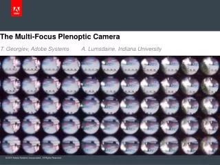
Kodacolor Plenoptic 1.0 camera capturing color was made by Kodak (1928) Using black and white film
1.0 Super-Resolution • In both 1.0 and 2.0 we superresolve the same way: • - Effectively shear the radiance • integral projection • This interleaves pixel from neighboring microimages, increasing resolution: • In 1.0 we need to shear a lot more than in 2.0, also need to deconvolve.
2.0 Super-Resolution In 2.0 camera we shear less. That’s because radiance is captured sheared. Example with no shear: The difference: In 2.0 pixels are already in focus. They “fit in” exactly. No need for deconvolution. Because of that quality is better.
Super-Demosaic • The color filters from the Bayer array are equivalent to spacing between pixels • in each individual color channel. • Algorithm: • First effectively shear the raw data to the right location • Then do integral projection and demosaic • This gains you 4 times better resolutioncompared to • the traditional “demosaic, then superresolve.” • Note: There is no real shearing in the above superresolution algorithms. Shearing is “effective” in the sense that we are achieving the effect of shearing by appropriate sampling when “adding up” pixels for the integral projection.
Raw sampled data directly from the CCD Raw plenoptic 2.0 data before color demosaic
Live demo in the poster session Super-Demosaic