Download
1 / 43
430 likes | 559 Vues
Instruction and Data Address Trace Compression. Aleksandar Milenković (collaborative work with Milena Milenković and Martin Burtscher) Electrical and Computer Engineering Department The University of Alabama in Huntsville Email: milenka@ece.uah.edu Web: http://www.ece.uah.edu/~milenka

E N D
Instruction and Data Address Trace Compression Aleksandar Milenković (collaborative work with Milena Milenković and Martin Burtscher) Electrical and Computer Engineering Department The University of Alabama in Huntsville Email: milenka@ece.uah.edu Web: http://www.ece.uah.edu/~milenka http://www.ece.uah.edu/~lacasa
Outline • Program Execution Traces • Trace Compression • Trace Compression in Hardware • Stream caches and predictors for instruction address trace compression • Data address stride caches for data address trace compression • Results • Conclusions
Program Execution Traces • Streams of recorded events • Basic block traces • Address traces • Instruction words • Operands • Trace uses • Computer architects for evaluation of new architectures • Computer analysts for workload characterization • Software developers for program tuning, optimization, and debugging
Instruction and Data Address Traces:An Example for(i=0; i<100; i++) { c[i] = s*a[i] + b[i]; sum = sum + c[i]; } Dinero+ Execution Trace DataAddress InstructionAddress Type @ 0x020001f4: mov r1,r12, lsl #2 @ 0x020001f8: ldr r2,[r4, r1] @ 0x020001fc: ldr r3,[r14, r1] @ 0x02000200: mla r0,r2,r8,r3 @ 0x02000204: add r12,r12,#1 (1 >>> 0) @ 0x02000208: cmp r12,#99 (99 >>> 0) @ 0x0200020c: add r6,r6,r0 @ 0x02000210: str r0,[r5, r1] @ 0x02000214: ble 0x20001f4 2 0x020001f4 0 0x020001f8 0xbfffbe24 0 0x020001fc 0xbfffbc94 2 0x02000200 2 0x02000204 2 0x02000208 2 0x0200020c 1 0x02000210 0xbfffbb04 2 0x02000214
Trace Issues • Trace issues • Capture • Compression • Processing • Traces tend to be very large • In terabytes for a minute of program execution • Expensive to store, transfer, and use • Effective reduction techniques: • Lossless • High compression ratio • Fast decompression
Outline • Program Execution Traces • Trace Compression • Trace Compression in Hardware • Stream caches and predictors for instruction address trace compression • Data address stride caches for data address trace compression • Results • Conclusions
Trace Compression • General purpose compression algorithms • Ziv-Lempel (gzip) • Burroughs-Wheeler transformation (bzip2) • Sequitur • Trace specific compression techniques • Tuned to exploit redundancy in traces • Better compression, faster, can be further combined with general-purpose compression algorithms
Trace-Specific Compression Techniques Lossless Compression Instructions Instructions + data Link data addresses to dynamic basic block Offset Mache [Samples 1989],LBTC [Luo and John 2004] Replacing an execution sequence with its identifier [Pleszkun 1994],SBC [Milenkovic and Milenkovic, 2003] Offset + repetitions • Acyclic path (WPP [Larus 1999], Time Stamped WPP [Zhang and Gupta 2001]) • - N-tuple [Milenkovic, Milenkovic and Kulick 2003] • Instruction (PDI [Johnson, Ha and Zaidi 2001]) Control flow graph + trace of transitions PDATS [Johnson, Ha and Zaidi 2001] Link data addresses to loop QPT [Larus 1993] [Elnozahy 1999], SIGMA [DeRose, et al. 2002] Regenerate addresses Abstract execution Value Predictor Graph with number of repetitions in nodes VPC [Burtscher and Jeeradit 2003],TCGEN [Burtscher and Sam 2005] [Eggers, et al. 1990],[Larus 1993] [Hamou-Lhadj and Lethbridge 2002]
Outline • Program Execution Traces • Trace Compression • Trace Compression in Hardware • Stream caches and predictors for instruction address traces • Data address stride caches for data address traces • Results • Conclusions
Why Trace Compression in Hardware? • Problem #1: Capture program traces • In software: trap after each instruction or taken branch • E.g., IBM’s Performance Inspector • Slowdown > 100 times • Multiple cores on a single chip + more detailed information needed (e.g., time stamps of events) • Problem #2: debugging is far from fun • Stop execution on breakpoints, examine the state • Time-consuming, difficult, may miss a critical state leading to erroneous behavior • Stopping the CPU may perturb the sequence of events making your bugs disappear • => Need an unobtrusive real-time tracing mechanism
Trace Compression in Hardware • Goals • Small on-chip area and small number of pins • Real-time compression (never stall the processor) • Achieve a good compression ratio • Solution • A set of compression algorithms targeting on-the-fly compression of instruction and data address traces
Exploiting Stream and Strides • Instruction address trace compression • Limited number andstrong temporal locality of instruction streams • => Replace an instruction streamwith its identifier • Data address trace compression • Spatial and temporal locality of data addresses • => Recognize regular strides
PC DA Trace Compressor: System Overview Processor Core Data Address Task Switch Program Counter System Under Test Data AddressBuffer Processor Core Memory Stream Cache(SC) Data Address Stride Cache (DASC) Trace Compressor SCIT SCMT DMT DT Predictor +Byte rep. FSM Byte rep.FSM Trace port External Trace Unitfor Storing/Processing (PC or Intelligent Drive) Trace Output Controller To External Unit
Outline • Program Execution Traces • Trace Compression • Trace Compression in Hardware • Stream caches and predictors for instruction address traces • Data address stride caches for data address traces • Results • Conclusions
0x020001f4 0x020001f8 ... 0x02000214 PC PPC SA SL - Instruction Stream Buffer =! 4 S.SA S.L Stream Detector + Stream Cache Stream Cache (SC) NWAY - 1 … iWay 1 0 0 1 F(S.SA, S.SL) 0x0E i S.SA & S.L iSet ’00…0’ iWay (0x020001f4,0x09) NSET - 1 S.SA & S.LFrom InstructionStream Buffer =? Hit/Miss 0x00 // it. 0 SCMT (SA, SL) SCIT (0x020001f4,0x09) Stream Cache Index Trace Stream Cache Miss Trace 0x0E // it. 1 0x0E // it. 99
Instruction Stream Buffer size Not to stall processor (e.g., have consecutive very short instruction streams) Stream cache Size Associativity Replacement policy Mapping function SC Itrace Compression Compress instruction stream Get the next instruction stream record from the instruction stream buffer(S.SA, S.SL); Lookup in the stream cache with iSet = F(S.SA, S.SL); if (hit) Emit(iSet && iWay) to SCIT; else { Emit reserved value 0 to SCIT; Emit stream descriptor (S.SA, S.SL) to SCMT; Select an entry (iWay) in the iSet set to be replaced; Update stream cache entry: SC[iSet][iWay].Valid = 1 SC[iSet][iWay].SA = S.SA, SC[iSet][iWay].SL = S.SL;} Update stream cache replacement indicators; Design Decisions:
SC Itrace Compression: An Analytical Model Legend: • CR(SC.I) – compression ratio • N – number of instructions • SL.Dyn – average stream length (dynamic) • SC.Hit(Nset,Nway) – SC hit rate • Assumptions: • stream length < 256(1 byte for SL) • 4 bytes for stream starting address
2nd Level Itrace Compression • Size(SCIT) >> Size(SCMT) • HitRate = 98%, 8-bit index => Size(SCIT) = 10*Size(SCMT) • Redundancy in SCIT • Temporal and spatial locality of instruction streams • Reduce SCIT trace • Global Predictor • N-tuple compression using Tuple History Table • N-tuple compression using SCIT History Buffer
Global Predictor Structure SCIT Trace History Buffer Predictor next.sid 0 F pindex MaxP-1 ==? ’0’ ’1’ Hit/Miss SCIT PRED Trace SCIT PRED Miss Trace
Length of history buffer SCIT Compression Predict SCIT index Get the incoming index, next.sid, from the SCIT trace Calculate the SCIT predictor index, pindex, using indices in the History bufferpindex = F (indices in the History Buffer); Perform lookup in the SCIT Predictor with pindex; if(SCIT.Predictor[pindex] == next.sid) Emit(‘1') to SCIT PRED trace; else { Emit(‘0’) to SCIT PRED trace; Emit next.sid to SCIT Miss PRED trace; SCIT.Predictor[pindex] = next.sid; } Shift in the next.sid to the History Buffer; Design Decisions: • Global predictor • Size • Mapping function
Redundancy in SCIT Pred Trace • High predictor hit rates and long runs of 0xFF bytes are expected in Predictor Hit Trace • Use a simple FSM to exploit byte repetitions PREDHit Trace // Detect byte repetitions in SCIT pred 1. Get next SCIT Pred byte, Next.BYTE; 2. if (Next.BYTE == Prev.BYTE) CNT++; 3. else { 4. if (CNT == 0) { 5. Emit Prev.BYTE to SCIT.REP.Trace; 6. Emit ‘0’ to SCIT Header; 7. } else { 8. Emit (Prev.BYTE, CNT) pair to SCIT.REP.Trace; 9. Emit ‘1’ to SCIT Header;} 10. Prev.BYTE = Next.BYTE;} Prev.BYTE CNT =? SCIT PRED Repetition Trace SCIT PRED Header
Outline • Program Execution Traces • Trace Compression • Trace Compression in Hardware • Stream caches and predictors for instruction address traces • Data address stride caches for data address traces • Results • Conclusions
Data Address Trace Compression • More challenging task • Data addresses rarely stay constant during program execution • However, they often have a regular stride • => Use Data Address Stride Cache (DASC) to exploit locality of memory referencing instructions and regularity in data address strides
Data Address Stride Cache Data Address Stride Cache (DASC) 0x020001f8 DASC • Tagless structure • Indexed by PC of the corresponding instruction • Entry fields • LDA – Last Data Address • Stride PC 0 1 G(PC) i index 0xbfffbe24 N - 1 0xbfffbe20 0xbfffbe1c DA DA-LDA ==? ’0’ ’1’ Stride.Hit Stride.Hit 0xbfffbe24 DT (Data trace) DMT Data Miss Trace 0xbfffbe20 0 1 0
Number of entries Index function G Stride length Data address buffer depth DASC Compression // Compress data address stream Get the next pair from data buffers (PC, DA) Lookup in the data address stream cache indexSet = G(PC); cStride = DA - DASC[iSet].LDA; if (cStride == DASC[iSet].Stride) { Emit(‘1’) to DT; //1-bit info } else { Emit(‘0’) to DT; Emit DA to DMT; DASC[iSet].Stride =lsb(cStride);} DASC[iSet].LDA = DA; Design Decisions:
DASC Dtrace Compression: An Analytical Model Legend: • CR(SC.D) – compression ratio • Nmemref – number of memory referencing instructions • DASC.Hit – DASC hit rate • Assumptions: • 4 bytes for stream starting address
Redundancy in DT Trace • High predictor hit rates and long runs of 0xFF bytes are expected in DT Trace • Use a simple FSM to exploit byte repetitions DT // Detect data repetitions 1. Get next DT byte; 2. if (DT == Prev.DT) CNT++; 3. else { 4. if (CNT == 0) { 5. Emit Prev.DT to DRT; 6. Emit ‘0’ to DH; 7. } else { 8. Emit (Prev.DT, CNT) pair to DRT; 9. Emit ‘1’ to DH;} 10. Prev.DT = DT;} Prev.DT CNT =? Data Header (DH) Data Repetition Trace (DRT)
Outline • Program Execution Traces • Trace Compression • Trace Compression in Hardware • Stream caches and predictors for instruction address traces • Data address stride caches for data address traces • Results • Conclusions
Experimental Evaluation • Goals • Assess the effectiveness of the proposed algorithms • Explore the feasibility of the proposed hardware implementations • Determine optimal size and organization of HW structures • Workload • 16 MiBench benchmarks • ARM architecture • Legend: • IC – Instruction count • NUS – Number of unique instruction streams • maxSL – Maximum stream length • SL.Dyn – Average stream length (dynamic)
Findings about SC Size/Organization • Good compression ratio • Outperforms fast GZIP • High stream cache hit rates for all application (>98 %) • Smaller SCs work well too • Replacement policy • Pseudo-LRU vs. FIFO • Associativity • 4-way is a reasonable choice • 8-way and 16-way desirable • Mapping function • S.SA<5+n:6> xor S.L<n-1:0>n=log2(NSET)
Findings about Global Predictor • Number of entries should not exceed the number of entries in SC • Having longer histories and larger predictorsgives only marginal improvements for all applicationsexcept ghostscript, blowfish, and stringsearch • History length = 1 • Index GPRED using the previous SCIT index
Findings about DASC • Stride size • 1 byte is optimal • 2 byte stride improves compression for 10% • DASC with 1K entriesis an optimal choice • Tagged (multi-way) DASC further improves overall compression ratio • Increased complexity
Hardware Complexity Estimation • CPU model • In-order, Xscale like • Vary SC and DASC parameters • SC and DASC timings • SC: Hit latency = 1 clock, Miss latency = 2 clocks • DASC: Hit latency = 2 clocks Miss latency = 2 clocks • To avoid any stalls • Instruction stream input buffer: MIN = 2 entries • Data address input buffer: MIN = 8 entries • Results are relatively independent of SC and DASC organization
Outline • Program Execution Traces • Trace Compression • Trace Compression in Hardware • Stream caches and predictors for instruction address traces • Data address stride caches for data address traces • Results • Conclusions
Conclusions • A set of algorithms and hardware structuresfor instruction and data address trace compression • Stream Caches + Global Predictor + Byte repetition FSMfor instruction traces • Data Address Stride Cache + Byte repetition FSM for data traces • Benefits • Enabling real-time trace compression with high compression ratio • Low complexity (small structures, small number of external pins) • Analytical & simulation analysis focusing on compression ratio and optimal sizing/organization of the structures as well as real-time trace port bandwidth requirements
Laboratory for Advanced Computer Architectures and Systems at Alabama: Research Overview Aleksandar Milenković The LaCASA Laboratory Electrical and Computer Engineering Department The University of Alabama in Huntsville Email: milenka@ece.uah.edu Web: http://www.ece.uah.edu/~milenka http://www.ece.uah.edu/~lacasa
Secure Processors PMAC (Parallel MACs) for reducedcryptographic latency A variation of the one-time-pad for code encryption Instruction Verification Buffer for conditional execution before verification Software & physical attacks Computer Security is Critical Sign & Verify for Guaranteed Integrity and Confidentiality of Code Improvements http://www.ece.uah.edu/~lacasa/research.htm#secure_processors
Small programs for uncovering architectural parameters (usually not publicly disclosed) of modern processors Relatively simple, so their behavior can be understood Benefits Architecture-aware compiler optimization Processor design evaluation and verification Testing Competitive analysis Microbenchmarks for Architectural Analysis Microbenchmarks • Results • Microbenchmarks for BTB analysis • Experimental flow foroutcome predictor • Tested on P6 and NetBurst (Northwood core) BTB Size Outcome Predictor BTB Org. BTB BTB Indexing ... Local History PerformanceCounters • Challenge • Dothan (PentiumM) predictor Branch relatedevents Global History ... http://www.ece.uah.edu/~lacasa/bp_mbs/bp_microbench.htm
TinyHMS Prototype Concept Software http://www.ece.uah.edu/~lacasa/research.htm#tinyHMS
Motion Sensor(TS2) ECGSensor(TS1) Heart Beat Heart Beat Step Heart Beat Step BeaconMessage BeaconMessage Event Messagewith Timestamp … … TS2 TS2 TS3 TS3 NC NC TS1 TS1 Frame i Frame i-1 TinyHMS