Download
1 / 13
130 likes | 217 Vues
Blended Rain Rate. Stan Kidder 23 February 2010. Objective. To develop a Blended Rain Rate product, like the Blended TPW product, which will be of use to forecasters. Must combine as much satellite data as possible into one product Must be as timely (least latency) as possible

E N D
Blended Rain Rate Stan Kidder 23 February 2010
Objective To develop a Blended Rain Rate product, like the Blended TPW product, which will be of use to forecasters. • Must combine as much satellite data as possible into one product • Must be as timely (least latency) as possible • Must be as free as possible of distracting artifacts • Must be accessible to forecasters in formats and map projections that they can use (McIDAS, AWIPS)
How It Works Product Generation(DPEAS) Data Ingest( FTP from DDS) Web Server Product Archive
Data Ingest Andy Jones’s Chair Data Ingest
Everything Else Product Generation and Web Server Archive
DPEAS Processing Swath Processing Swath Ingest Application of Blending Algorithm Swath Mapping Compositing
5-Day Histograms (of raining pixels) 1.0 0.25 OCEAN “LAND” SSM/I 0.25 mm/hr bins MHS PDF PDF AMSU-B 0.0 0.0 0 0 2 2 4 4 6 6 8 8 10 10 Rain Rate (mm/hr) SSM/I shows expected “lognormal” distribution, but AMSU-B and MHS do not Over “land” all PDFs are similar
Cumulative PDF 1.0 CPDF Interpolate CPDFs to correct RR OCEAN 0.0 Rain Rate (mm/hr) 0 2 4 6 8 10 Corrected RR Input RR
The Algorithm • No correction over land (=“not ocean”) • No correction for SSM/I • For AMSU-B and MHS over ocean • No correction for RR > 5 mm/hr • Only negative corrections allowed • All scan positions treated the same • DMSP F13 SSM/I is the “reference satellite” • Fortunately, I captured DMSP F13 histograms to be used in the event of its failure • Linearly interpolate the CPDFs to get correction
All AMSU-B or MHS Before Note lack of rain rates below 0.5 mm/hr Too much blue and green
After AMSU-B or MHS SSM/I AMSU-B and MHS look a lot more like SSM/I than they would have without correction