Download
1 / 34
400 likes | 689 Vues
Properties of Populations. D ensity. Age structure. Fertility. What is a population?. A group of organisms of the same species that occupy a well defined geographic region and exhibit reproductive continuity from generation to generation; ecological

E N D
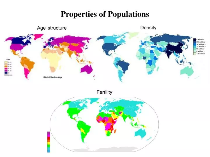
Properties of Populations Density Age structure Fertility
What is a population? • A group of organisms of the same species that occupy a well defined geographic • region and exhibit reproductive continuity from generation to generation; ecological • and reproductive interactions are more frequent among these individuals than with • members of other populations of the same species. Population 1 Population 2
A local example: Pinus ponderosa Geographic distribution of P. ponderosa • Broken up into populations • But they are messy!
In the real world, defining populations isn’t simple • Populations often do not have clear boundaries • Even in cases with clear boundaries, movement may be common Habitat 2 Habitat 1
An extreme example…Ensatinasalamanders Not only are populations continuous, but so are species!
Metapopulations make things even more complicated • Occur in fragmented habitats • Connected by limited migration • Characterized by extinction • and recolonization • populations are transient
Glanville Fritillary in the Åland Islands The glanville fritillary Red dots indicate occupied patches and white dots empty patches in 1993. Picture by Timo Pakkala
Some Important Properties of Populations • 1) Density – The number of organisms per unit area • 2) Genetic structure – The spatial distribution of genotypes • 3) Age structure – The ratio of one age class to another • 4) Growth rate – (Births + Immigration) – (Deaths + Emigration)
Describing populations I – Population density United States at night Population density of the Carolina wren • Population density shapes: • Strength of competition within species • Spread of disease • Strength of interactions between species • Rate of evolution
Population density and disease, Trypanasoma cruzi (Chagas disease) Trypanasoma cruzi (protozoan) Currently infects between 16,000,000 and 18,000,000 people and kills about 50,000 people each year “Assassin bug” (vector)
Population density and disease, Trypanasoma cruzi A case study from the Brazilian Amazon • Since 1950, human population has increased ≈ 7 fold • Since 1950, the number of infections has increased ≈ 30 fold • Suggests that rates of infection are increasing with human density Antonio R.L. Teixeira, et. al., 2000. Emerging infectious diseases. 7: 100-112.
Describing populations II – Genetic structure Imagine a case with 2 alleles: A and a, with frequencies pi and qi, respectively aa AA AA aa AA aa Aa aa AA AA AA aa AA Aa aa Aa aa AA Aa aa p1 = .9 p2 = .1 Population 1 Population 2 p2 = 2/20 = .1 q2 = 18/20 = .9 = 1-p2 p1 = 18/20 = .9 q1 = 2/20 = .1 = 1-p1 These populations exhibit genetic structure!
Sickled cells and malaria resistance Malaria in red blood cells A ‘sickled’ red blood cell
Global distribution of Malaria and the Sickle cell gene Recently colonized by malaria; low frequency of sickle allele Historical range of malaria; high frequency of sickle allele The frequency of the sickle cell gene is higher in populations where Malaria has been prevalent historically
What determines a population’s age structure? • Probability of death for various age classes • Probability of reproducing for various age classes • These probabilities are summarized using life tables
Mortality schedules: the probability of dying at age x Parental care Number surviving (Log scale) Little parental care Age
Proportion surviving to age x Quantifying mortality using life tables Number alive at age x Age class How could you collect this data in a natural population? Now let’s work through calculating the entries
Calculating entries of the life table: lx The proportion surviving to age class x = The probability of surviving to age class x lx = Nx/N0 Follow a single ‘cohort’
What determines a population’s age structure? • Probability of death for various age classes • # of offspring produced by various age classes • These probabilities are summarized using life tables
Fecundity schedules – # of offspring produced at age x mx = The expected number of daughters produced by mothers of age x Some mammals mx Long lived plants Age
Fertility schedules can also be summarized in life tables This entry designates the EXPECTED # of offspring produced by an individual of age 4. In other words, this is the AVERAGE # of offspring produced by individuals of age 4
If lx and mx do not change, populations reach a stable age distribution Population starting with all four year olds High juvenile but low adult mortality Population starting with all one year olds Low juvenile but high adult mortality As long as lx and mxremain constant, these distributions would never change!
Describing populations IV – Growth rate Negative growth Positive growth Zero growth A population’s growth rate can be readily estimated *** if a stable age distribution has been reached ***
Using life tables to calculate population growth rate The first step is to calculate R0: R0 = ∑ lx mx This number, R0, tells us the expected number of offspring produced by an individual over its lifetime. • If R0 < 1, the population size is decreasing • If R0 = 1, the population size is steady • If R0 > 1, the population size is increasing R0 = ∑ lx mx = 1*0 + .75*0 + .5*1 + .25*4 = 1.5
Using life tables to calculate population growth rate The second step is to calculate G This number, G, is a measure of the generation time of the population, or more specifically, the expected or average age of reproduction
Using life tables to calculate population growth rate The last step is to calculate r This number, r, is a measure of the population growth rate. Specifically, r is the probability that an individual gives birth per unit time minus the probability that an individual dies per unit time. Population growth rate depends on two things: 1. Generation time, G 2. The number of offspring produced by each individual over its lifetime, R0
The importance of generation time Imagine two different populations, each with the same R0: Population 2 Population 1 R0,2 = 1.5 R0,1 = 1.5 G2 = 1.33 G1 = 3.67 r1 = .110 r2 = .305 The growth rate of population 2 is almost three times greater, even though individuals in the two populations have identical numbers of offspring!
Using r to predict the future size of a population The change in population size, N, per unit time, t, is given by this differential equation: Using basic calculus Gives us an equation that predicts the population size at any time t,Nt,for a current population of size N0: One of the most influential equations in the history of biology
What are the consequences of this result? For population size to remain the same, the following must be true: This is the concept of anequilibrium This can only be true if ???
What are the consequences of this result? If r is anything other than 0 (R0 is anything other than 1), the population goes extinct or becomes infinitely large r = 0 r = .1 r = -.1 Population size, N Generation Generation Generation
A real example of exponential population growth… From 0-1500: Human population increases by ≈ 1.0 billion From 1500-2000: Human population increases by ≈ 10.0 billion This observation had important historical consequences…
Using life tables: A practice question A team of conservation biologists is interested in determining the optimum environment for raising an endangered species of flowering plant in captivity. For their purposes, the optimum environment is the one that maximizes the growth rate of the captive population allowing more individuals to be released into the wild in each generation. To this end, they estimated life table data for two cohorts (each of size 100) of captive plants, each raised under a different set of environmental conditions. Using the data in the hypothetical life tables below, answer the following questions: A. Using the data from the hypothetical life tables above, calculate the expected number of offspring produced by each individual plant over its life, R0, for each of the populations. B. Using the data in the life tables above, calculate the generation time for each of the populations. C. Using your calculations in A and B, estimate the population growth rate, r, of the two populations. Which population is growing faster? Why? D. Assuming the populations both initially contain 100 individuals, estimate the size of each population in five years. E. If the sole goal of the conservation biologists was to maximize the growth rate of the captive population, which conditions (those experienced by population 1 or 2) should they use for their future programs? *** We will work through this problem during the next class. Be prepared***