Download
1 / 69
700 likes | 884 Vues
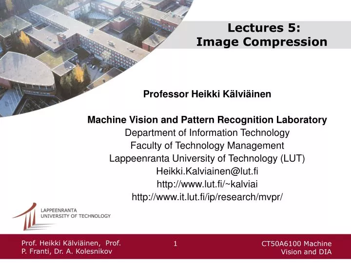
Lectures 5: Image Compression. Professor Heikki Kälviäinen Machine Vision and Pattern Recognition Laboratory Department of Information Technology Faculty of Technology Management Lappeenranta University of Technology (LUT) Heikki.Kalviainen@lut.fi http://www.lut.fi/~kalviai

E N D
Lectures 5: Image Compression • Professor Heikki Kälviäinen • Machine Vision and Pattern Recognition Laboratory • Department of Information Technology • Faculty of Technology Management • Lappeenranta University of Technology (LUT) • Heikki.Kalviainen@lut.fi • http://www.lut.fi/~kalviai • http://www.it.lut.fi/ip/research/mvpr/ Prof. Heikki Kälviäinen, Prof. P. Franti, Dr. A. Kolesnikov
Content • Introduction. • Fundamentals in data compression. • Binary Image Compression. • Continuous tone images. • Video image compression. • The material at the following site are used: • http://cs.joensuu.fi/pages/franti/imagecomp/ • Special thanks to the authors of the material • Prof. Pasi Fränti and • Dr. Alexander Kolesnikov • from University of Joensuu, Finland. Prof. Heikki Kälviäinen, Prof. P. Franti, Dr. A. Kolesnikov
Introduction • Why do we need to compress images? • Image types. • Parameters of digital images. • Lossless vs. lossy compression. • Measures: rate, distortion, etc. Prof. Heikki Kälviäinen, Prof. P. Franti, Dr. A. Kolesnikov
What is data and image compression? Data compression is the art and science of representing information in a compact form. Data is a sequence of symbols taken from a discrete alphabet. Still image data, that is a collection of 2-D arrays (one for each color plane) of values representing intensity (color) of the point in corresponding spatial location (pixel). Prof. Heikki Kälviäinen, Prof. P. Franti, Dr. A. Kolesnikov
Why do we need image compression? Still image: • One page of A4 format at 600 dpi is > 100 MB. • One color image in a digital camera generates 10-30 MB. • Scanned 3”7” photograph at 300 dpi is 30 MB. Digital cinema: • 4K2K3 12 bits/pel = 48 MB/frame or 1 GB/sec or 70 GB/min. Prof. Heikki Kälviäinen, Prof. P. Franti, Dr. A. Kolesnikov
Why do we need image compression? (cont.) 1) Storage. 2) Transmission. 3) Data access. 1990-2000 Disc capacities : 100MB -> 20 GB (200 times!) but seek time : 15 milliseconds 10 milliseconds and transfer rate : 1MB/sec ->2 MB/sec. Compression improves overall response time in some applications. Prof. Heikki Kälviäinen, Prof. P. Franti, Dr. A. Kolesnikov
Source of images • Image scanner. • Digital camera. • Video camera. • Ultra-sound (US), Computer Tomography (CT), Magnetic resonance image (MRI), digital X-ray (XR), Infrared. • Etc. Prof. Heikki Kälviäinen, Prof. P. Franti, Dr. A. Kolesnikov
Image types Why do we need special algorithms for images? Prof. Heikki Kälviäinen, Prof. P. Franti, Dr. A. Kolesnikov
Binary image: 1 bit/pixel Prof. Heikki Kälviäinen, Prof. P. Franti, Dr. A. Kolesnikov
Grayscale image: 8 bits/pixel Intensity = 0-255 Prof. Heikki Kälviäinen, Prof. P. Franti, Dr. A. Kolesnikov
Parameters of digital images Prof. Heikki Kälviäinen, Prof. P. Franti, Dr. A. Kolesnikov
True color image: 3*8 bits/pixel Prof. Heikki Kälviäinen, Prof. P. Franti, Dr. A. Kolesnikov
RGB color space RedGreenBlue Prof. Heikki Kälviäinen, Prof. P. Franti, Dr. A. Kolesnikov
YUV color space Y U V Prof. Heikki Kälviäinen, Prof. P. Franti, Dr. A. Kolesnikov
RGB YUV R, G, B -- red, green, blue Y -- theluminance U,V -- the chrominance components Most of the information is collected to the Y component, while the information content in the U and V is less. Prof. Heikki Kälviäinen, Prof. P. Franti, Dr. A. Kolesnikov
Palette color image Look-up-table [R,G,B] = LUT[Index] Example: [64,64,0] = LUT[98] Prof. Heikki Kälviäinen, Prof. P. Franti, Dr. A. Kolesnikov
Multicomponent image: n*8 bits/pixel • Spectral image: • n components • according to • wavelengths. Three components R, G, B => “usual” color image. Prof. Heikki Kälviäinen, Prof. P. Franti, Dr. A. Kolesnikov
Multicomponent image: n*8 bits/pixel (cont.) • Spectral components and spatial components. For example, remote sensing (satellite images). Prof. Heikki Kälviäinen, Prof. P. Franti, Dr. A. Kolesnikov
Why we can compress image? • Statistical redundancy: 1) Spatial correlation a) Local: pixels at neighboring locations have similar intensities. b) Global: reoccurring patterns. 2) Spectral correlation – between color planes. 3) Temporal correlation – between consecutive frames. • Tolerance to fidelity: (toistotarkkuus) 1) Perceptual redundancy. 2) Limitation of rendering hardware. Prof. Heikki Kälviäinen, Prof. P. Franti, Dr. A. Kolesnikov
Lossy vs. lossless compression Lossless compression: reversible, information preserving text compression algorithms, binary images, palette images. Lossy compression: irreversible grayscale, color, video. Near-lossless compression: medical imaging, remote sensing. 1) Why do we need lossy compression? 2) When we can use lossy compession? Prof. Heikki Kälviäinen, Prof. P. Franti, Dr. A. Kolesnikov
Lossy vs. lossless compression (cont.) Prof. Heikki Kälviäinen, Prof. P. Franti, Dr. A. Kolesnikov
What measures? • Bit rate: How much per pixel? • Compression ratio: How much smaller? • Computation time: How fast? • Distortion: How much error in the presentation? Prof. Heikki Kälviäinen, Prof. P. Franti, Dr. A. Kolesnikov
Rate measures Bit rate: bits/pixel Compression ratio: k = the number of bits per pixel in the original image C/N = the bit rate of the compressed image Prof. Heikki Kälviäinen, Prof. P. Franti, Dr. A. Kolesnikov
Distortion measures Mean average error (MAE): Mean square error (MSE): Signal-to-noise ratio (SNR): (decibels) Pulse-signal-to-noise ratio (PSNR): (decibels) A is amplitude of the signal: A = 28-1=255 for 8-bits signal. Prof. Heikki Kälviäinen, Prof. P. Franti, Dr. A. Kolesnikov
Other issues • Coder and decoder computation complexity. • Memory requirements. • Fixed rate or variable rate. • Error resilience (sensitivity). • Symmetric or asymmetric. • Decompress at multiple resolutions. • Decompress at various bit rates. • Standard or proprietary (application based). Prof. Heikki Kälviäinen, Prof. P. Franti, Dr. A. Kolesnikov
Fundamentals in data compression • Modeling and coding: • How, and in what order the image is processed? • What are the symbols (pixels, blocks) to be coded? • What is the statistical model of these symbols? • Requirement: • Uniquely decodable: different input => different output. • Instantaneously decodable: the symbol can be recognized after its last bit has been received. Prof. Heikki Kälviäinen, Prof. P. Franti, Dr. A. Kolesnikov
Modeling: Segmentation and order of processing • Segmentation: • Local (pixels) or global (fractal compression). • Compromise: block coding. • Order of processing: • In what order the blocks (or the pixels) are processed? • In what order the pixels inside the block are processed? Prof. Heikki Kälviäinen, Prof. P. Franti, Dr. A. Kolesnikov
Modeling: Order of processing • Order of processing: • Row-major order: top-to-down, left-to-right. • Zigzag scanning: • Pixel-wise processing (a). • DCT-transformed block (Discrete Cosine Transform) (b). • Progressive modeling: • The quality of an image quality increases gradually as data are received. • For example in pyramid coding: first the low resolution version, then increasing the resolution. Prof. Heikki Kälviäinen, Prof. P. Franti, Dr. A. Kolesnikov
Modeling: Order of processing Prof. Heikki Kälviäinen, Prof. P. Franti, Dr. A. Kolesnikov
Modeling: Statistical modeling Set of symbols (alphabet) S={s1, s2, …, sN}, N is number of symbols in the alphabet. Probability distribution of the symbols: P={p1, p2, …, pN} According to Shannon, the entropy H of an information source S is defined as follows: Prof. Heikki Kälviäinen, Prof. P. Franti, Dr. A. Kolesnikov
Modeling: Statistical modeling The amount of information in symbol si, i.e., the number of bits to code or code length for the symbol si: The average number of bits for the source S: Prof. Heikki Kälviäinen, Prof. P. Franti, Dr. A. Kolesnikov
Modeling: Statistical modeling • Modeling schemes: • Static modeling: • Static model (code table). • One-pass method: encoding. • ASCII data: p(‘e’)= 10 %, p(‘t’)= 8 %. • Semi-adaptive modeling: • Two-pass method: (1) analysis, (2) encoding. • Adaptive (or dynamic) modeling: • Symbol by symbol on-line adaptation during coding/encoding. • One-pass method: analysis and encoding. Prof. Heikki Kälviäinen, Prof. P. Franti, Dr. A. Kolesnikov
Modeling: Statistical modeling • Modeling schemes: • Context modeling: • Spatial dependencies between the pixels. • For example, what is the most probable symbol after a known sequence of symbols? • Predictive modeling (for coding prediction errors): • Prediction of the current pixel value. • Calculating the prediction error. • Modeling the error distribution. • Differential pulse code modulation (DPCM). Prof. Heikki Kälviäinen, Prof. P. Franti, Dr. A. Kolesnikov
Coding: Huffman coding INIT: Put all nodes in an OPEN list and keep it sorted all times according to their probabilities. REPEAT a) From OPEN pick two nodes having the lowest probabilities, create a parent node of them. b) Assign the sum of the children’s probabilities to the parent node and inset it into OPEN. c) Assign code 0 and 1 to the two branches of the tree, and delete the children from OPEN. Prof. Heikki Kälviäinen, Prof. P. Franti, Dr. A. Kolesnikov
Huffman Coding: Example Symbol pi -log2(pi) Code Subtotal A 15/39 1.38 0 2*15 B 7/39 2.48 100 3*7 C 6/39 2.70 101 3*6 D 6/39 2.70 110 3*6 E 5/39 2.96 111 3*5 Total: 87 bits Binary tree 1 0 A 0 1 H = 2.19 bits L = 87/39=2.23 bits 1 0 1 E B D C Prof. Heikki Kälviäinen, Prof. P. Franti, Dr. A. Kolesnikov
Huffman Coding: Decoding A - 0 B - 100 C - 101 D - 110 E - 111 Bit stream: 1000100010101010110111 (22 bits) Codes: 100 0 100 0 101 0 101 0 110 111 Message: B A B A C A C A D E 1 0 A 0 1 Binary tree 1 0 1 E B D C Prof. Heikki Kälviäinen, Prof. P. Franti, Dr. A. Kolesnikov
Properties of Huffman coding • Optimum code for a given data set requires two passes. • Code construction complexity O(N log N). • Fast lookup table based implementation. • Requires at least one bit per symbol. • Average codeword length is within one bit of zero-order entropy (Tighter bounds are known): H R H+1 bit • Susceptible to bit errors. Prof. Heikki Kälviäinen, Prof. P. Franti, Dr. A. Kolesnikov
Coding: Arithmetic coding • Alphabet extension (blocking symbols) can lead to coding efficiency. • How about treating entire sequence as one symbol! • Not practical with Huffman coding. • Arithmetic coding allows you to do precisely this. • Basic idea: map data sequences to sub-intervals in [0,1) with lengths equal to the probability of corresponding sequence. • QM-coder is an arithmetic coding tailored for binary data. • 1) Huffman coder: H R H + 1 bit/pel • 2) Block coder: Hn Rn Hn + 1/n bit/pel • 3) Arithmetic coder: H R H + 1 bit/message (!) Prof. Heikki Kälviäinen, Prof. P. Franti, Dr. A. Kolesnikov
Arithmetic coding: Example 0.70 Prof. Heikki Kälviäinen, Prof. P. Franti, Dr. A. Kolesnikov
Binary image compression • Binary images consist only of two colors, black and white. • The probability distribution of the alphabet is often very skew: p(white)=0.98, and p(black)=0.02. • Moreover, the images usually have large homogenous areas of the same color. Prof. Heikki Kälviäinen, Prof. P. Franti, Dr. A. Kolesnikov
Binary image compression: Methods • Run-length encoding. • Predictive encoding. • READ code. • CCITT group 3 and group 4 standards. • Block coding. • JBIG, JBIG2 (Joint Bilevel Image Experts Group). • Standard by CCITT and ISO. • Context-based compression pixel by pixel. • QM-coder (arithmetic coder). Prof. Heikki Kälviäinen, Prof. P. Franti, Dr. A. Kolesnikov
Run-length coding: Idea • Pre-processing method, good when one symbol occurs with high probability or when symbols are dependent. • Count how many repeated symbol occur. • Source ’symbol’ = length of run. Example: …, 4b, 9w, 2b, 2w, 6b, 6w, 2b, ... Prof. Heikki Kälviäinen, Prof. P. Franti, Dr. A. Kolesnikov
Run-length encoding: CCITT standard Huffman code table Prof. Heikki Kälviäinen, Prof. P. Franti, Dr. A. Kolesnikov
JBIG Bilevel (binary) documents. Both graphics and pictures (halftone). Graphic (line art) Halftone Prof. Heikki Kälviäinen, Prof. P. Franti, Dr. A. Kolesnikov
Comparison of algorithms Prof. Heikki Kälviäinen, Prof. P. Franti, Dr. A. Kolesnikov
Continuous tone images: lossless compression • Lossless and near-lossless compression. • Bit-plane coding: to bit-planes of a grayscale image. • Lossless JPEG (Joint Photographic Experts Group). • Pixel by pixel by predicting the current pixel on the basis of the neighboring pixels. • Prediction errors coded by Huffman or arithmetic coding (QM-coder). Prof. Heikki Kälviäinen, Prof. P. Franti, Dr. A. Kolesnikov
Continuous tone images: lossy compression • Vector quantization: codebooks. • JPEG (Joint Photographic Experts Group). • Lossy coding of continuous tone still images (color and grayscale). • Based on Discrete Cosine Transform (DCT): • 0) Image is divided into block NN. • 1) The blocks are transformed with 2-D DCT. • 2) DCT coefficients are quantized. • 3) The quantized coefficients are encoded. Prof. Heikki Kälviäinen, Prof. P. Franti, Dr. A. Kolesnikov
JPEG: Encoding and Decoding Prof. Heikki Kälviäinen, Prof. P. Franti, Dr. A. Kolesnikov
Divide image into NN blocks Input image 8x8 block Prof. Heikki Kälviäinen, Prof. P. Franti, Dr. A. Kolesnikov
2-D DCT basis functions: N=8 Low High Low Low 8x8 block High High High Prof. Heikki Kälviäinen, Prof. P. Franti, Dr. A. Kolesnikov Low