Download

1 / 52
520 likes | 761 Vues
Reducing NoC Energy Consumption Through Compiler-Directed Channel Voltage Scaling. Guangyu Chen, Feihui Li, Mahmut Kandemir, Mary Jane Irwin Microsystems Design Lab, Department of CSE The Pennsylvania State University mdl@cse.psu.edu. Why NoCs?. Scalability

E N D
Reducing NoC Energy Consumption Through Compiler-Directed Channel Voltage Scaling Guangyu Chen, Feihui Li, Mahmut Kandemir, Mary Jane Irwin Microsystems Design Lab, Department of CSE The Pennsylvania State University mdl@cse.psu.edu
Why NoCs? • Scalability • Support for large number of processing units • Flexibility • Topology and routing policy can be configured according to the needs of a particular application • Point-to-point, broadcasting (one-to-multiple), gathering (multiple-to-one) • Performance • Low latency, high bandwidth • Reliability • Multiple routes between a source/target pair • Signal strengthening in routers PLDI’06
Mesh-Based NoC Abstraction Communication Channel Router CPU CPU CPU Memory Memory Memory CPU CPU CPU Memory Memory Memory CPU CPU CPU Memory Memory Memory PLDI’06
Related Work • Communication channels can account for a significant portion to the chip energy consumption (between 20% and 45%) • Prior efforts • Simunic and Boyd: NoC power modeling (DATE’02) • Benini and De Micheli: Design methodology for energy-efficient reliable SoC networks (ISSS’01) • Shang et al: Hardware-directed DVS for communication links (HPCA’03) • Kim et al: Communication link shutdown (ISLPED’03) • Soteriou and Peh: Design space exploration for link turn on/off (ICCD’04) • Soteriou et al: Software-directed power-aware interconnection networks (CASES’05) • Li et al: Software-directed DVS for communication links (CASES’05) • Li et al: Compiler-directed link turnoff and routing (ICCAD’05, EMSOFT’05, POPL’06) • Our goal is to save network energy through voltage/frequency scaling PLDI’06
Motivational Example (1) Node 2 Node 1 for i = 0 to N { send(2, A[i][0..1023] receive(2, buffer) } for i = 0 to N{ send(1, A[i][0..255] receive(1, buffer) } i=0 i=1 i=2 i=3 i=4 PLDI’06
Node 1 Node 2 Motivational Example (2) Node 2 Node 1 for i = 0 to N { send(2, A[i][0..255] short computation receive(2, buffer) } for i = 0 to N{ send(1, A[i][0..255] long computation receive(1, buffer) } Node 1 Node 2 i=4 i=0 i=1 i=2 i=3 PLDI’06
Process and Connection Mapping • NoC Parameters Overview of Our Approach CriticalPathAnalysis BuildingIPCG InputParallel Code IPCG CodeModification Scaling Factorfor EachConnection OutputParallelCode PLDI’06
Assumptions • Array-based embedded applications • Message-passing based parallel program • For each send(p, m) instruction, the destination node p, and the size of message m can be statically determined at compilation time • For each receive(p, m) instruction, the source node p can be determined at compilation time • A send instruction is blocked if the previous message send by the same node has not been delivered to the destination node • A receive instruction is blocked if the message is not ready in the buffer of the receiver node • Code is parallelized and process-to-node mapping is performed • Network is exposed to the compiler PLDI’06
Inter-Process Communication Graph (IPCG) • IPCG G(P) captures the communication behavior of application P • G(P) = (V(P), E(P), , ) • V(P): the set of vertices • E(P): the set of edges • , : the weights for edges, capturing minimum/maximum execution latencies PLDI’06
Vertices of IPCG • V(P) = X(P) B(P) S(P) D(P) R(P) • x X(P): the entry point of a loop in program P • b B(P): the back jump of a loop in program P • s S(P): the point in P at which a message is sent • d D(P): the point in P at which a message is delivered • r R(P): the point in P at which a message is used send(2,..) Node 1 s Node 2 d r messagedelivered receive(1,..) PLDI’06
Edges of IPCG • Task edges • Communication edge (s, d): a message is sent at point s S(P) and delivered at point d D(P) • Computation edge (u, v): a computation task starts at point u and ends at point v • u, v X(P) S(P) R(P) • Control edges • Enforce the order at which the points of the given program can be reached • Back-jump edge • Other control edges PLDI’06
and Functions • (u,v) and (u,v): the minimum and maximum times required to execute task (u,v) • For communication edge (s,d) • (s,d) = (min. message size) / (max. data rate) • (u,v) = (max. message size) / (max. data rate) • For computation edge (u, v) • (s,d) = the minimum time for executing the instructions between u and v • (u,v) = the maximum time for executing the instructions between u and v • For control edge(u,v) • (s,d) = (u,v) = 0 PLDI’06
IPCG Example (1) // Process 1 x3:for(...) { r1:receive(2,..) 20–25 cycles s2:send(2,..) } // Process 2 x1:for(...) { s1:send(1,..); x2:for(...) { 10 cycles s3:send(3,..); 10–15 cycles s4:send(3,..); 80-90 cycles r5:receive(3,..) 20 cycles } r2:receive(1,..); } // Process 3 x4:for(...) { 10 cycles r3:receive(2,..) 15 cycles r4:receive(2,..) 40-50 cycles s5:send(2,..) } PLDI’06
IPCG Example (2) x4 10/10 10/10 10/10 0/0 x3 x1 s3 d3 r3 0/0 15/15 10/15 s1 d1 r1 s4 r4 d4 0/0 10/15 20/25 10/15 x2 40/50 80/90 s2 120/ s5 d5 r5 d2 r2 0/0 10/10 0/0 10/10 20/20 b3 0/0 b4 b2 b1 p2 p3 p1 PLDI’06
IPCG Example (2) x4 x3 x1 s3 d3 r3 s1 d1 r1 s4 r4 d4 x2 s2 s5 d5 r5 d2 r2 b3 b4 b2 b1 p2 p3 p1 PLDI’06
IPCG Example (2) x4 x3 x1 s3 d3 r3 s1 d1 r1 s4 r4 d4 x2 s2 s5 d5 r5 d2 r2 b3 b4 b2 b1 p2 p3 p1 PLDI’06
IPCG Example (2) x4 x3 x1 s3 d3 r3 s1 d1 r1 s4 r4 d4 x2 s2 s5 d5 r5 d2 r2 b3 b4 b2 b1 p2 p3 p1 PLDI’06
IPCG Example (2) x4 x3 x1 s3 d3 r3 s1 d1 r1 s4 r4 d4 x2 s2 s5 d5 r5 d2 r2 b3 b4 b2 b1 p2 p3 p1 PLDI’06
IPCG Example (2) x4 10/10 x3 x1 s3 d3 r3 s1 d1 r1 s4 r4 d4 10/15 10/15 x2 s2 s5 d5 r5 d2 r2 10/10 10/10 b3 b4 b2 b1 p2 p3 p1 PLDI’06
IPCG Example (2) x4 10/10 10/10 10/10 0/0 x3 x1 s3 d3 r3 0/0 15/15 10/15 s1 d1 r1 s4 r4 d4 0/0 10/15 20/25 10/15 x2 40/50 80/90 s2 120/ s5 d5 r5 d2 r2 0/0 10/10 0/0 10/10 20/20 b3 0/0 b4 b2 b1 p2 p3 p1 PLDI’06
IPCG Example (2) x4 10/10 10/10 10/10 0/0 x3 x1 s3 d3 r3 0/0 15/15 10/15 s1 d1 r1 s4 r4 d4 0/0 10/15 20/25 10/15 x2 40/50 80/90 s2 120/ s5 d5 r5 d2 r2 0/0 10/10 0/0 10/10 20/20 b3 0/0 b4 b2 b1 p2 p3 p1 PLDI’06
IPCG Example (2) x4 10/10 10/10 10/10 0/0 x3 x1 s3 d3 r3 0/0 15/15 10/15 s1 d1 r1 s4 r4 d4 0/0 10/15 20/25 10/15 x2 40/50 80/90 s2 120/ s5 d5 r5 d2 r2 0/0 10/10 0/0 10/10 20/20 b3 0/0 b4 b2 b1 p2 p3 p1 PLDI’06
IPCG Example (2) x4 10/10 10/10 10/10 0/0 x3 x1 s3 d3 r3 0/0 15/15 10/15 s1 d1 r1 s4 r4 d4 0/0 10/15 20/25 10/15 x2 40/50 80/90 s2 120/ s5 d5 r5 d2 r2 0/0 10/10 0/0 10/10 20/20 b3 0/0 b4 b2 b1 p2 p3 p1 PLDI’06
x4 10/10 10/10 10/10 0/0 x3 x1 s3 d3 r3 0/0 15/15 10/15 s1 d1 r1 s4 r4 d4 0/0 10/15 20/25 10/15 x2 40/50 80/90 s2 120/ s5 d5 r5 d2 r2 0/0 10/10 0/0 10/10 20/20 b3 0/0 b4 b2 b1 p2 p3 p1 IPCG Example (2) PLDI’06
A set of loops that communicate with each other Unit of granularity for optimization Parallel Loop Group x4 10/10 10/10 10/10 0/0 x3 x1 s3 d3 r3 0/0 15/15 10/15 s1 d1 r1 s4 r4 d4 0/0 10/15 20/25 10/15 x2 40/50 80/90 s2 120/ s5 d5 r5 d2 r2 0/0 10/10 0/0 10/10 20/20 b3 0/0 b4 b2 b1 PLDI’06
R = 3 q = 1 Q = 4 j = 0 j = 1 j = 2 j = 3 j = 4 j = 5 j = 6 j = 7 j = 8 t1,0 t1,1 t1,2 t1,3 t1,4 t1,5 t1,6 t1,7 t1,8 Loop x1 t2,0 t2,1 t2,2 t2,3 t2,4 t2,5 t2,6 t2,7 t2,8 Loop x2 t3,0 t3,1 t3,2 t3,3 t3,4 t3,5 t3,6 t3,7 t3,8 Loop x3 t4,0 t4,1 t4,2 t4,3 t4,4 t4,5 t4,6 t4,7 t4,8 Loop x4 T T Representative Iterations • A set of loop iterations that represent the timing behavior of the entire parallel loop group Time PLDI’06
Critical Path Analysis • Determine q and Q such that [q, Q– 1] are the set of representative loop iterations • Determine t[i,j]: the earliest time that node vi at the jth iteration (j [q, Q-1]) can be reached, assuming each task is completed in the shortest time • Determine t[i,j]: the earliest time that node vi at the jth iteration (j [q, Q-1]) can be reached, assuming each task takes the longest time • Determine the scaling factor for each communication channel such that the overall performance degradation due to voltage scaling is within (a preset bound) PLDI’06
Determining t[i,j] - Constraints where : the set of intra-iteration edges : at each iteration j, u must be reached before v : the set of inter-iteration edges : u at the (j – 1)th iteration must be reached before v at the jth iteration PLDI’06
Examples of Intra- and Inter-Iteration Edges x4 x3 x1 s3 d3 r3 s1 d1 r1 s4 r4 d4 x2 s2 s5 d5 r5 d2 r2 b3 b4 b2 b1 p2 p3 p1 Intra-Iteration edge Inter-Iteration edge PLDI’06
Determining t[i,j] - Example x2 x3 x1 d3 s2 s3 s1 d1 d1 20/25 20/25 20/25 25/30 20/20 20/25 r2 r3 r1 25/30 15/15 10/10 b2 b3 b1 p2 p3 p1 PLDI’06
t[s1,0] + (s1, d1)t[d1, 0] 0+20=20 Determining t[i,j] - Example 20 PLDI’06
Determining t[i,j] - Example PLDI’06
Determining t[i,j] - Example PLDI’06
Determining t[i,j] – Example q = 2, Q = 4, T = 50 PLDI’06
Determining t[i,j] - Constraints where : the set of intra-iteration edges : the set of inter-iteration edges PLDI’06
Determining Scaling Factor -Constraints where : the set of intra-iteration and inter-iteration edges : the node that executes operation v : the maximum performance degradation allowed : the scaling factor for the network connection from node n1 to n2 We try to maximizek(n1, n2) for each connection PLDI’06
Determining Scaling Factor - Algorithm repeat select a connection C scale down the data rate of C by one grade determine t[i, j] using if make the data rate of C permanent else restore the data rate of C until no more connection can be scale down PLDI’06
Determining Scaling Factor - Example q = 2, Q = 4, T = 100, = 10%, k = 1, 0.8, 0.6, 0.4, 0.2 PLDI’06
Determining Scaling Factor - Example q = 2, Q = 4, T = 100, = 10%, k = 1, 0.8, 0.6, 0.4, 0.2 k[1, 2] = 0.8, k[2, 3] = 1, k[3, 1] = 1 PLDI’06
Determining Scaling Factor - Example q = 2, Q = 4, T = 100, = 10%, k = 1, 0.8, 0.6, 0.4, 0.2 k[1, 2] = 0.8, k[2, 3] = 0.8, k[3, 1] = 1 PLDI’06
Determining Scaling Factor - Example q = 2, Q = 4, T = 100, = 10%, k = 1, 0.8, 0.6, 0.4, 0.2 k[1, 2] = 0.8, k[2, 3] = 1, k[3, 1] = 0.8 PLDI’06
Determining Scaling Factor - Example q = 2, Q = 4, T = 100, = 10%, k = 1, 0.8, 0.6, 0.4, 0.2 k[1, 2] = 0.6, k[2, 3] = 1, k[3, 1] = 1 PLDI’06
Determining Scaling Factor - Example q = 2, Q = 4, T = 100, = 10%, k = 1, 0.8, 0.6, 0.4, 0.2 k[1, 2] = 0.4, k[2, 3] = 1, k[3, 1] = 1 PLDI’06
Determining Scaling Factor - Example q = 2, Q = 4, T = 100, = 10%, k = 1, 0.8, 0.6, 0.4, 0.2 k[1, 2] = 0.2, k[2, 3] = 1, k[3, 1] = 1 PLDI’06
Determining Scaling Factor - Example q = 2, Q = 4, T = 100, = 10%, k = 1, 0.8, 0.6, 0.4, 0.2 k[1, 2] = 0.2, k[2, 3] = 1, k[3, 1] = 1 RESULT:k[1, 2] = 0.4, k[2, 3] = 1, k[3, 1] = 1 PLDI’06
Shared Communication Channels The voltage level of the channel shared by multiple connections is determined by the connection that requires the highestvoltage level v1 a c v1 v3 v2 v2 v2 b b v3 v1 v3 v1 c a PLDI’06
Experimental Setup PLDI’06
Impact on Energy Consumption PLDI’06
Energy Consumption Breakdown PLDI’06
Accuracy of Voltage Selection PLDI’06