Download
1 / 20
200 likes | 452 Vues
Acoustic Based Angle-Of-Arrival Estimation in the Presence of Interference. Andrew McMurdie and Wanyang Zhang Electrical Engineering Department Brigham Young University. Sound-detection Based System. Two audio mirrors and the audio wall at Denge , in Kent, England.

E N D
Acoustic Based Angle-Of-Arrival Estimation in the Presence of Interference Andrew McMurdie and Wanyang Zhang Electrical Engineering Department Brigham Young University
Sound-detection Based System Two audio mirrors and the audio wall at Denge, in Kent, England. Image provided courtesy of the Geograph Britain and Ireland Project.
Acoustic Location and Sound Mirrors The height-locating half of the Czech four-horn acoustic locator. Image provided courtesy of The Museum of Retro Technology.
Angle of Arrival Equation Δt = =
Proposed Acoustic Detection System • Power received is given by: • Where Pg is the power generated by the source (in Watts of sound power), Ar is the area of the receiver (in square meters), and R is the one way range from the source to the listening station. • Assumes that the microphones are lossless (100% efficient), that the receiver is ideal, and that the signal processing of the system causes no further losses from the source to the listening station.
Initial System Performance • With no noise, maximum range of aircraft is 28,209 km • GPS Satellites orbit at 20,000 km • Obviously unrealistic, because of simple acoustics model chosen
Simulation Setup • Cars on highway 100 m behindlistening stations • Beyond -1km and 1km, cars are in tunnel – no noise to listeningstations • Listening stations 50 m apart • Aircraft flies in circle with centerbetween listening stations
Noise Modeling • The number of car arrivals into the range of received stations in each second obeys a Poisson distribution • The noise of each car generated is modeled as white noise • Car sound power is 77 dBW at source • Assume worst-case scenario – all phases add together • Average power at receivers is 39 dBW
Cars On Highway During Simulation • Cars take 68.5 seconds to traverse highway • Expected value is 140 cars
Aircraft Signal Modeling • Jetliner engine with sound power of 160dBW • Airplane engine recorded sound • Aircraft sound is assumed to repeat every second • Sound is assumed to be known at the receiver
SNR Considerations • Correlation becomes more unreliable with falling SNR • System requirement is 90% probability of detection • Empirically found to be possible at zero dB SNR • At -1 dB, probability of detection is 88% • At -3 dB, probability of detection is 87% • At -7 dB, probability of detection is 50% • At -10 dB, probability of detection is 20%
Maximum Range with Noise • With noise power of 39 dBand required zero dB SNR,maximum range is found tobe 313.6 km • Still unrealistic • International Space Stationorbits at 320 km at lowest point • This is Low-Earth Orbit • Max range is just over 1% ofthat with no noise
Simulation Execution • Run in MATLAB • Required 7000 seconds – just over an hour and a half for full flight • Speed of sound taken into consideration • Assumed a constant 340.29 m/s • Long delay times in getting sound from aircraft to receiver stations • No Doppler assumed
Simulation At Longer Range • Want to test empirical observation of probability of detection • Range set to result in -3dB SNR at listening stations – 443.5 km • Required simulation time of 8000 seconds (because of longer flight arc)
Simulation Results at -3dB SNR • System has multiplemissed detections • Angular response of system is greatly degraded • Best performance at -30to +30 degrees
Conclusions • Model very basic; ranges are unrealistic • Demonstrates the deficiencies of an acoustic-based detection system • Plane velocity > Mach 1 • Long time delay • Acoustic detection systems better when targets known to have very low velocities, need passive sensors • Simulation shows worst-case scenario; average performance may be better
Questions/ Comments?