Statistical Modeling and Data Analysis Given a data set, first question a statistician ask is,

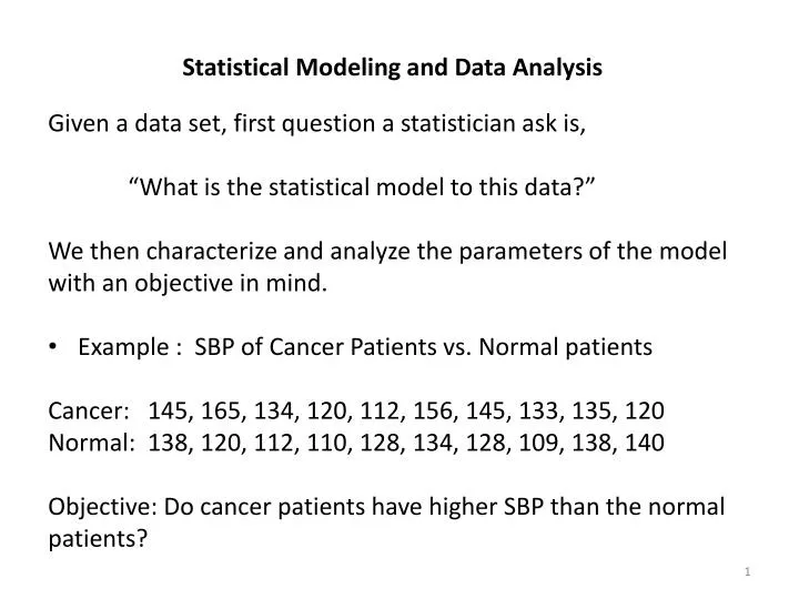
1. Statistical Modeling and Data Analysis • Given a data set, first question a statistician ask is, • “What is the statistical model to this data?” • We then characterize and analyze the parameters of the model with an objective in mind. • Example : SBP of Cancer Patients vs. Normal patients • Cancer: 145, 165, 134, 120, 112, 156, 145, 133, 135, 120 • Normal: 138, 120, 112, 110, 128, 134, 128, 109, 138, 140 • Objective: Do cancer patients have higher SBP than the normal patients?

2. Population of cancer patients with a probability distribution Population of normal patients with a probability distribution normal cancer Systolic blood pressure Objective is to test the Hypothesis: Does the data support this hypothesis?

3. Assumption: The data is random and is generated from the normal distributions? • Random Variable • is the collection of all subjects. What we observe is one realization • Random Sample: • We collect a sample of subjects

4. Observed Sample: • Assumption: – Simple Random Sample • (equally likely than any other sample) • Multivariate Observations • An observed vector is one realization of this, i.e.,

5. Random Sample: Observed sample is a realization of Note: If the simultaneous inference is to made on its components, the probability statement should be viewed in terms of probability of observing

6. Stochastic Process Observed value of this is one realization Can we describe a probability distribution of ? Kolmogorov Consistency Theorem says that probability distribution can be described.

7. These are three realizations with

8. Discrete time points If this process is stationary, then a probability model for can be described in a concise way. For example, , where is white noise.

9. Image Process:

10. , where is the set of all pixels. Note that what we observe is a realization of this

11. The same can be said about weather map.

12. Data Analysis • Generally speaking, we perform one or more of the following tasks in data analysis (statistical inference) • Estimate the model • Hypothesis testing • Predictive analysis • Given the sample data, objective is to make inference about the population described by the probability model. • All inferences are based on probability model assumed.

13. Estimation Think of estimating any parameters of a probability model. For example, estimating and of a regression model How good is the estimate ? Well, you might say that if , it is a good estimate. Not so simple! Note that is unknown.

14. Frequentist’s Interpretation Note that depends on the sample we observe. is better than if the average of is smaller than the average of , i.e., for all .

15. is better than if for all . A best estimate, in this sense, is of course not possible. If irrespective of the observed sample, then for We restrict to a class of estimators, and then try to find best Estimate within this class. For example, we may consider a class of all unbiased estimators.

16. Theories are well developed for achieving best estimates among the class of unbiased estimates for simple probability models. For complicated model, we can always fall back to maximum likelihood estimates. Obtain the estimate by maximizing the likelihood function For small sample size , this may not always yield good estimate, but for large sample size , this generally yield optimal estimates.

17. Asymptotic Optimality of Maximum Likelihood Estimate – sequence of asymptotically normal estimates as can be interpreted as asymptotic variance of . , - Fisher Information Matrix Under regular probability models, maximum likelihood estimates achieves the lower bound.

18. Bayesian Interpretation Prior Distribution - Through this we might say that some values of are more likely than other values. is better than if . A best estimate is now possible; for example, The RHS is the expectation with respect to the posterior distribution of .

19. Prior Distribution - Really? Where did it come from? You may not believe this, but we are really talking in terms of a statistical philosophy. Can you really believe that the true state of nature is random? normal cancer Systolic blood pressure

20. and are supposed to be fixed mean SBPs of the normal and cancer populations. Now, we are saying that they are random. Bayesian Paradigm is never a fixed value; under most circumstances some values of are more likely than other values. Before a data is analyzed, we should explore this prior. Then update it based on the information provided by the data. Prior: Data: Posterior: All information about is contained in the posterior.

21. Example: 1 in 1,000 in the population carry a particular genetic disorder. Certain tests on a person are performed, and data is collected Data: Prior: Posterior:

22. The main issues with Bayesian inference are (1) Appropriateness of the prior (2) Computation of the posterior distribution random sample from Prior: This is a conjugate prior because the posterior distribution is of same form as the prior distribution. Is this prior appropriate?

23. Prior: If nothing is known about , . This gives almost flat prior for and . There are other ways to assign non-informative priors. Note that if Prior: then we will have computational problem of computing posterior distribution.

24. Computation of the posterior There are two popular techniques of computing posterior distribution: 1. Metropolis-Hasting Algorithm 2. Gibbs Sampler These techniques can be used effectively for complex probability model and reasonable priors.

25. Frequentist vs. Bayesian FrequentistBayesian All data information is All data information is contained in the likelihood contained in the likelihood function. function and the prior The estimates are viewed Estimates are viewed in in terms of how they behave terms of where they are on the average located in the posterior Estimates are generally obtained Estimates are obtained from by maximizing the likelihood the posterior. Techniques function. Techniques include include Gibbas Sampler, Newton-Raphson, EM-algorithm Metropolis-Hasting etc.

26. Mixture Models Suppose the population is a mixture of two or more populations. Bayesians would have a good answer to estimate this model than frequentists would.

27. Hypothesis Testing Think about how it started in statistical literature. Data: drawn from a probability model. associated with the probability model Does the data support this hypothesis? Bayesians had an answer to this, but they were not popular at the time. Ans.

28. (Fisher) drawn from Hypothesis : Compute If this is vey small (, then the data provide very little evidence in support of the hypothesis. Conclusion: Reject the Hypothesis

29. Analysis of Variance (ANOVA) ANOVA is one of the most popular statistical tools of analyzing data. Factor 1 Y Factor 2 A Response Variable Factor 3 Does Y (the response) depends on any of the factors?

30. Example 1: You are doing a research on mpg (miles per gallon) for a brand of automobiles. Question: What effects mpg? Wind speed mpg Air temperature Air moisture Do wind speed, air temperature, and air moisture effect mpg?

31. Example 2: Research Question: Does blood pressure (BP) depend on weight and gender? Weight BP Gender

32. There is a variation in BP. Some is due to weight, and some is due to gender. * Female * Male * ** * * * * * * * BP * * Weight

33. Concept: Variation(BP) = Variation(Weight) + Variation(Gender) + Variation(Error) These variation can be described by Sums of Squares SS(BP) = SS(Weight) + SS(Gender) + SS(Error) is the degrees of freedom that represent the effective number of terms in the sums of squares

34. F-Statistics Weight: Test Statistic Hypothesis : Weight is not a factor in BP If p-value (<0.05), then there is little evidence that weight is not a factor Gender: Test Statistics Same can be done to see if gender is a factor.

35. Neyman – Pearson Lemma Basis for Classical Hypothesis Testing Null hypothesis Alternative Hypothesis (Research Hypothesis) TS: Test Statistics Decision Rule Conclusion Type-I Error: False Discovery Type-II Error: False Non-Discovery Devise a decision rule so that = Pr(False Discovery) is very small (=0.05). Through Neyman-Pearson Lemma, a most powerful decision rule can be obtained.

36. Uniformly Most Powerful Unbiased Decision Rule is , where is such that . Note that this is a frequentist method since the probability statement should be interpreted in a frequentist manner.

37. Likelihood Approach Neyman-Perason Lemma works only on simple probability models. Test Statistics If the hypothesis is correct, the should be closed to 0. Thus, we reject the hypothesis if The cut-off point can be obtained through asymptotic distribution of , which is usually .

38. Model Selection Suppose you want choose one model out of several. This is a type of multiple hypotheses problem. Regression: Not all predictors are significant, and you want to select the set of significant predictors. This can be viewed as selecting one of the several models Choose the model that yields the smallest

39. This yields a biased selection, meaning that a model with higher number of parameters has a better chance of being selected. AIC or BIC Information criteria Select the model with the highest value of AIC (or BIC)

40. Bayesian Hypothesis Testing Data: drawn from Hypothesis Prior: Posterior: , Bayes Factor: If this Bayes factor (, data has sufficient evidence to support the hypothesis .

41. Frequentist Vs. Bayesian Note that both and classical hypothesis tests are frequentists since the statements are made in terms of probability. The Bayes Factor is used in Bayesian tests which is based on the posterior probability

42. Multiple Hypotheses: Consider 1000 independent tests each at Type-error of α = 0.05. Then 5% of the null hypotheses would be falsely rejected. In other words, if 50 of the hypotheses were rejected, there is no guarantee that they were not all falsely rejected. FWER: m = # of hypotheses π = P(One or more falsely rejected hypotheses) = 1 – (Bonferroni Correction)

43. If m is large, α would be very small. Thus the power of detecting any true positive would be very small. • Sequential Bonferroni Corrections: • Let be the p-values of independent tests with • corresponding null hypotheses . • Holm’s Method (Holm, 1979; Scand. Statist.) • If , accept all nulls. • If , reject ; if , accept the rest of nulls. • Continue until first j such that . In that case reject • all and accept the rest of nulls.

44. Simes Method (Biometrika, 1986): • If , reject all nulls. • If not, but if , reject all • Continue until first . In that case reject all Note: Both Holm’s and Simes methods are designed to refine the FWER.

45. False Discovery Rate (FDR): Benjaminiand Hochberg (1995), JRSS When the number of hypotheses m is very large (say in thousands), and if each individual hypothesis is not important, then FWER criterion is not very useful since it yields few discoveries. For example, in a microarray data analysis, the objective is to detect potential genes for future exploration. Here, each individual gene is not important. In such cases, tests with a controlled FWER would yield few discoveries.

46. FDR = Expected proportion of false rejections. FDR = = Note that FWER = P(R>0)

47. Benjamini and Hochberg proved that the following procedure produces : Let k be the largest integer i such that , then reject all The result was proved under the assumption of independent test statistics. It was later extended to a positively correlated test statistics by Benjamini and Yekutieli, 2001; Ann. Stat.

48. Bayesian Interpretation (Storey, 2003, Ann. Stat.) are independently distributed. Note: pFDR is a posterior version of the Type-I error

49. Directional Hypothesis Problem (Three decision problem): Suppose is rejected, but it is also important to find the direction of So the problem is to find subsets

50. Example: Gene selection When the genes are altered under adverse condition, such as cancer, the affected genes show under or over expression in a microarray. The objective is to find the genes with under expressions and genes with over expressions.