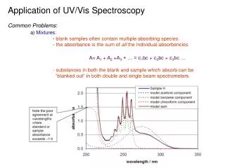
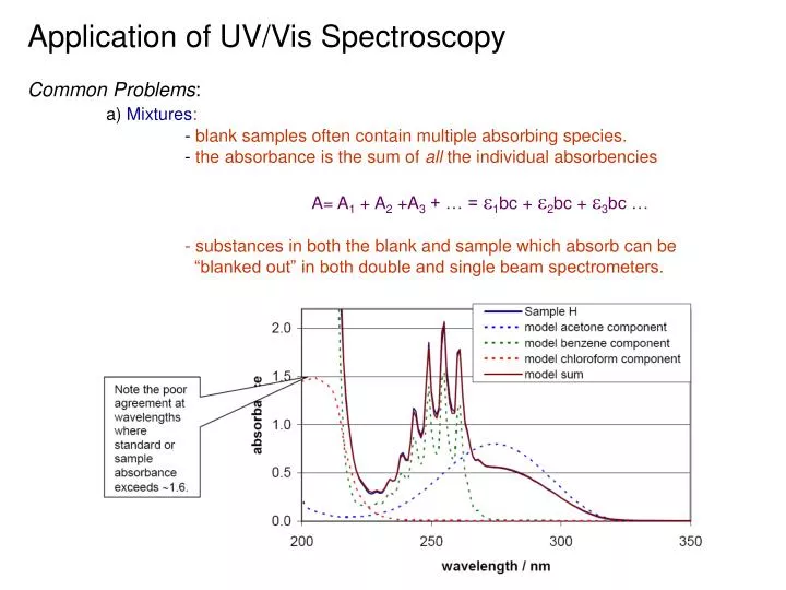
Application of UV/Vis Spectroscopy Common Problems : a) Mixtures :

1. Application of UV/Vis Spectroscopy Common Problems: a) Mixtures: - blank samples often contain multiple absorbing species. - the absorbance is the sum of all the individual absorbencies A= A1 + A2 +A3 + … = e1bc + e2bc + e3bc … - substances in both the blank and sample which absorb can be “blanked out” in both double and single beam spectrometers.

2. But, If the blank absorbance is high, Po will decrease too much, the response will be slow and the results inaccurate If blank absorbance too high: - dilute the sample - use a different l where the analyte absorbs more relative to the interference. - use a different method of separation Large blank absorbance l scan of substance

3. b) Instrumental Deviations from Beer’s Law: - stray light (already discussed). - polychromatic light (more then a single l) ‚since all instruments have a finite band pass, a range of l’s are sent through the sample. ‚e may be different for each l Deviation’s from Beer’s law at high concentration

4. Illustration of Deviation from Beer’s law: Let us say that exactly 2 wavelengths of light were entering the sample l = 254 nm e254 =10,000 l = 255 nm e255 = 5,000 let Po = 1 at both l’s What happens to the Beer’s law plot as c increases? A =A254 + A255 A = log Po/P (total) = log (Po254 + Po255)/(P254 + P255) At the individual l’s: A254 = e254bc = log Po254/P254 10ebc = Po254/P254 P254 = Po/10ebc = Po10-ebc For both together: A = log (Po254 + Po255)/(Po25410-e254bc + Po25510-e255bc)

5. Since Po254 = Po255 =1: A = 2.0/(Po25410-e254bc + Po25510-e255bc) A = 2.0/(10-10,000x1.0xc + 10-5000x1.0xc) The results are the same for more l’s of light. The situation is worse for greater differences in e’s (side of absorption peak, broad bandpass) Always need to do calibration curve! Can not assume linearity outside the range of linearity curve!

6. b) Chemical Deviations from Beer’s Law: - Molar absorptivity change in solutions more concentrated than 0.01M ‚due to molecular interactions ‚Beer’s law assumes species are independent ‚electrolytes may also cause this problem ‚e is also affected by the index of refraction - association, dissociation, precipitation or reaction of analyte ‚c in Beer’s law is the concentration of the absorbing species ‚commonly use the analytical concentration – concentration of all forms of the species. Ka phenolphthalein: H+ + In- HIn Red, l =600nm colorless If solution is buffered, then pH is constant and [HIn] is related to absorbance.

7. But, if unbuffered solution, equilibrium will shift depending on total analyte concentration Ka example: if Ka = 10-4 H+ + In- HIn “Apparent” deviation since can be accounted for by chemical equilibrium

8. But, if unbuffered solution, equilibrium will shift depending on total analyte concentration Ka example: if Ka = 10-4 H+ + In- HIn Isosbestic point At the isosbestic point in spectra: A = eb([HIn] + [In-])

9. c) Non-constant b: - worse for round cuvettes - use parallel cuvettes to help B2 P2 P0 B1 P1 A = log10 Po/P = ebc

10. d) Instrument noise: noise - short term baseline fluctuations, which decrease the precision of the analysis ‚can not measure A precisely ‚the various sources of noise each cause some uncertainty in the absorbance measurement and can be treated as individual standard deviations. 1) 0%T noise: - noise when light beam is blocked - seldom important - typically ±0.01%T 2) Readout Precision: - especially with a meter - typically ±0.5%T  1-3% error in concentration 3) Shot Noise: - occurs when e- transfers across a junction (like the space between cathode & anode in PMT). - causes random fluctuations in current since individual e- arrive at random times - increases with increase current (%T). Especially bad above 95%T.

11. 4) Flicker Noise: - noise from the lamp due to intensity changes - important at high transmittances. 5) Cell positioning uncertainty: - not really noise, but affects precision - minor imperfections, scratches or dirt change %T - may be the major cause of imprecision

12. Taken together, these noise sources indicate that the intermediate absorbance and transmittance ranges should be used. - at low %T, 0%T, noise and readout precision are important - at high %T, shot and flicker noise are large. Keep A in range of 0.1 – 1.5 absorbance units (80 -3%T)

13. Applications: A) Molar Absorptivities (e) in UV-Vis Range: e=8.7 x 1019 PA P – transition probability (ranges from 0.1 to 1, for likely transitions) A – cross-section area of target molecule (cm2) - ~10-15 cm2 for typical organics - emax = 104 to 105 L/mol-cm - e < 103 – low intensity (P £ 0.01)

14. - For Compounds with Multiple Chromophores: ‚If greater then one single bond apart - e are additive - l constant CH3CH2CH2CH=CH2lmax= 184 emax = ~10,000 CH2=CHCH2CH2CH=CH2lmax=185 emax = ~20,000 ‚If conjugated - shifts to higher l’s (red shift) H2C=CHCH=CH2lmax=217 emax = ~21,000

15. Example 6: The equilibrium constant for the conjugate acid-base pair HIn + H2O H3O+ + In- Calculate the absorbance at 430 nm for an indicator concentration of 3.00x10-4 M K = 8.00x10-5 e = 0.755x103 e = 8.04x103

16. Applications: B) Absorbing Species in UV/Vis: 1)Electronic transitions involving organic compounds, inorganic compounds, complexes, etc. Basic process: M + hn M* 10-8 – 10-9s M*  M + heat (or fluorescence, light, or phosphorescence) or 10-8 – 10-9s M*  N (new species, photochemical reaction) Note: excited state (M*) is generally short and heat produced not generally measurable. Thus, get minimal disturbance of systems (assuming no photochemical reaction)

17. 2)Absorption occurs with bonding electrons. - E(l) required differs with type of bonding electron. - UV-Vis absorption gives some information on bonding electrons (functional groups in a compound. - Most organic spectra are complex ‚electronic and vibration transitions superimposed ‚absorption bands usually broad ‚detailed theoretical analysis not possible, but semi-quantitative or qualitative analysis of types of bonds is possible. ‚ effects of solvent & molecular details complicate comparison

18. - Single bonds usually too high excitation energy for most instruments (£185 nm) ‚vacuum UV ‚most compounds of atmosphere absorb in this range, so difficult to work with. ‚usually concerned with functional groups with relatively low excitation energies (190 £l £850 nm). - Types of electron transitions: i) s, p, n electrons Sigma (s) – single bond electron Low energy bonding orbital High energy anti-bonding orbital

19. Pi (p) – double bond electron Low energy bonding orbital High energy anti-bonding orbital Non-bonding electrons (n): don’t take part in any bonds, neutral energy level. Example:Formaldehyde

20. ‚s s* transition in vacuum UV ‚n s* saturated compounds with non-bonding electrons l ~ 150-250 nm e ~ 100-3000 ( not strong) ‚n p*, p  p* requires unsaturated functional groups (eq. double bonds) most commonly used, energy good range for UV/Vis l ~ 200 - 700 nm n p* : e ~ 10-100 p  p*: e ~ 1000 – 10,000

21. Absorption Characteristics of Some Common Chromophores

22. Other Examples of Some Common Chromophores

23. ii) d/f electrons (transition metal ions) ‚ Lanthanide and actinide series - electronic transition of 4f & 5f electrons - generally sharp, well-defined bands not affected by associated ligands ‚ 1st and 2nd transition metal series - electronic transition of 3d & 4d electrons - broad peaks Crystal-Field Theory • In absence of external field d-orbitals are identical • Energies of d-orbitals in solution are not identical • Absorption involves e- transition between d- orbitals • In complex, all orbitals increase in energy where orbitals along bonding axis are destabilized

24. Magnitude of D depends on: - charge on metal ion - position in periodic table - ligand field strength : I- < Br- < Cl- < F- < OH- < C2O42- ~ H2O < SCN- < NH3 < ethylenediamine < o-phenanthroline < NO2- < CN- D increases with increasing field strength, so wavelength decreases

25. iii) Charge Transfer Complexes ‚ Important analytically because of large e (> 10,000) ‚Absorption of radiation involves transfer of e- from the donor to orbital associated with acceptor - excited state is product of pseudo oxidation/reduction process ‚ Many inorganic complexes of electron donor (usually organic) & electron acceptor (usually metal) - examples: Iron III thiocyanate Iron II phenanthroline (colorless) (deep red color)

26. C) Qualitative Analysis: 1)Limited since few resolved peaks - unambiguous identification not usually possible. 2) Solvent can affect position and shape of curve. - polar solvents broaden out peaks, eliminates fine structure. Loss of fine structure for acetaldehyde when transfer to solvent from gas phase Also need to consider absorbance of solvent.

27. 2) Solvent can affect position and shape of curve. - polar solvents broaden out peaks, eliminates fine structure. (a) Vapor Loss of fine structure for 1,2,4,5-tetrazine as solvent polarity increases (b) Hexane solution (c) Aqueous

28. 3) Solvent can also absorb in UV-vis spectrum.

29. 3) Can obtain some functional group information for certain types of compounds.. - weak band at 280-290 nm that is shifted to shorter l’s with an increase in polarity (solvent) implies a carbonyl group. ‚acetone: in hexane, max = 279 nm ( = 15) in water, max = 264.5 nm - solvent effects due to stabilization or destabilization of ground or excited states, changing the energy gap. ‚since most transitions result in an excited state that is more polar than the ground state - 260 nm with some fine structure implies an aromatic ring. Benzene in heptane More complex ring systems shift to higher l’s (red shift) similar to conjugated alkenes

30. UV Spectral Nomenclature

31. C) Quantitative Analysis (Beer’s Law): 1)Widely used for Quantitative Analysis Characterization - wide range of applications (organic & inorganic) - limit of detection  10-4 to 10-5 M (10-6 to 10-7M; current) - moderate to high selectivity - typical accuracy of 1-3% ( can be ~0.1%) - easy to perform, cheap 2) Strategies a) absorbing species - detect both organic and inorganic compounds containing any of these species (all the previous examples)

32. b) non- absorbing species - react with reagent that forms colored product - can also use for absorbing species to lower limit of detection - items to consider: l, pH, temperature, ionic strength - prepare standard curve (match standards and samples as much as possible) Non-absorbing Species (colorless) reagent (colorless) Complex (red) When all the protein is bound to Fe3+, no further increase in absorbance. As Fe3+ continues to bind protein red color and absorbance increases.

33. Standard Addition Method (spiking the sample) - used for analytes in a complex matrix where interferences in the UV/Vis for the analyte will occur: i.e. blood, sediment, human serum, etc.. - Method: (1) Prepare several identical aliquots, Vx, of the unknown sample. (2) Add a variable volume, Vs, of a standard solution of known concentration, cs, to each unknown aliquot. Note: This method assumes a linear relationship between instrument response and sample concentration.

34. (3) Dilute each solution to an equal volume, Vt. (4) Make instrumental measurements of each sample to get an instrument response, IR.

35. (5) Calculate unknown concentration, cx, from the following equation. Note: assumes a linear relationship between instrument response and sample concentration. Where: S = signal or instrument response k = proportionality constant Vs = volume of standard added cs = concentration of the standard Vx = volume of the sample aliquot cx = concentration of the sample Vt = total volume of diluted solutions

36. c) Analysis of Mixtures - use two different l’s with different e’s A1 = e1MbcM + e1NbcN (l1) A2 = e2MbcM + e2NbcN (l2) Note: need to solve simultaneous equations

37. d) Photometric titration -can measure titration with UV-vis spectroscopy. - requires the analyte (A), titrant (T) or titration product (P) absorbs radiation

38. Example 7: Given: Calculate the concentrations of A and B in solutions that yielded an absorbance of 0.439 at 475 nm and 1.025 at 700 nm in a 2.50-cm cell.