Download
1 / 23
230 likes | 377 Vues
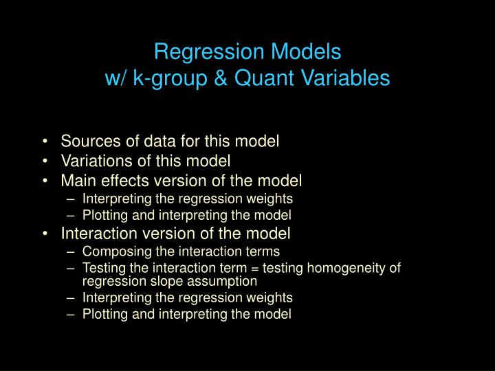
Regression Models w/ k-group & Quant Variables. Sources of data for this model Variations of this model Main effects version of the model Interpreting the regression weights Plotting and interpreting the model Interaction version of the model Composing the interaction terms

E N D
Regression Models w/ k-group & Quant Variables • Sources of data for this model • Variations of this model • Main effects version of the model • Interpreting the regression weights • Plotting and interpreting the model • Interaction version of the model • Composing the interaction terms • Testing the interaction term = testing homogeneity of regression slope assumption • Interpreting the regression weights • Plotting and interpreting the model
As always, “the model doesn’t care where the data come from”. Those data might be … • a measured k-group variable (e.g., single, married, divorced) and a measured quant variable (e.g., age) • a manipulated k-group variable (Tx1 vs. Tx2 vs. Cx) and a measured quant variable (e.g., age) • a measured k-group variable (e.g., single, married, divorced) and a manipulated quant variable (e.g., 0, 1, 2, 5,10 practices) • a manipulated binary k-group variable (Tx1 vs. Tx2 vs. Cx) and a manipulated quant variable (e.g., 0, 1, 2, 5, 10 practices) Like nearly every model in the ANOVA/regression/GLM family – this model was developed for and originally applied to experimental designs with the intent of causal interpretability !!! As always, causal interpretability is a function of design (i.e., assignment, manipulation & control procedures) – not statistical model or the constructs involved !!!
There are two important variations of this model • Main effects model • Terms for the k-group variable & quant variable • No interaction – assumes regression slope homgeneity • b-weights for k-group & quant variables each represent main effect of that variable • 2. Interaction model • Terms for k-group variable & quant variable • Term for interaction - does not assume reg slp homogen !! • b-weights for k-group & quant variables each represent the simple effect of that variable when the other variable = 0 • b-weight for the interaction term represented how the simple effect of one variable changes with changes in the value of the other variable (e.g., the extent and direction of the interaction)
Models with a centered quantitative predictor & a dummy coded k-category predictor This is called a main effects model there are no interaction terms. y’ = b1X + b2Z1+ b3Z2+ a Group Z1 Z2 1 1 0 2 0 1 3*0 0 • a regression constant • expected value of y if all predictors = 0 • mean of the control group (G3) • height of control group Y-X regression line • b1 regression weight for centered quant predictor • expected direction and extent of change in Y for a 1-unit increase in X after controlling for the other variable(s) in the model • main effect of X • slope of Y-X regression line for all groups • b2 regression weight for dummy coded comparison of G1 vs G3 • expected direction and extent of change in Y for a 1-unit increase in Z1, after controlling for the other variable(s) in the model • main effect of Z1 • Y-X reg line height difference for G1 & G3 • b3 regression weight for dummy coded comparison of G2 vs. G3 • expected direction and extent of change in Y for a 1-unit increase in Z2, after controlling for the other variable(s) in the model • main effect ofZ2 • Y-Xreg line height difference for G2 & G3
To plot the model we need to get separate regression formulas for each Z group. We start with the multiple regression model… Model y’ = b1X + b2Z1 + b3Z2 + a Group Z1 Z2 1 1 0 2 0 1 3*0 0 For the Comparison Group coded Z1= 0 & Z2 = 0 Substitute the Z code values y’ = b1X + b2*0 + b3*0 + a Simplify the formula y’ = b1X + a height slope For the Target Group coded Z1= 1 & Z2 = 0 Substitute the Z code values y’ = b1X + b2*1 + b3*0 + a Simplify the formula y’ = b1X + (b2 + a) height slope For the Target Group coded Z1= 0 & Z2 = 1 Substitute the Z code values y’ = b1X + b2*0 + b3*1 + a Simplify the formula y’ = b1X + (b3 + a) height slope
Plotting & Interpreting Models with a centered quantitative predictor & a dummy coded k-category predictor This is called a main effects model no interaction the regression lines are parallel. y’ = b1X + -b2Z1+ b3Z2+ a Xcen = X – Xmean Z1 = Tx1 vs. Cx(0) Z2 = Tx2 vs. Cx (0) a= ht of Cx line mean of Cx b1 = slp of Cx line b3 Tx2 Cx slp = Tx1 slp = Tx2 slp No interaction 0 10 20 30 40 50 60 Cx b1 -b2 b2= htdif Cx & Tx1 Cx & Tx1 mean dif Tx1 a b3= htdif Cx & Tx2 Cx & Tx2 mean dif -20 -10 0 10 20 Xcen
Plotting & Interpreting Models with a centered quantitative predictor & a dummy coded k-category predictor This is called a main effects model no interaction the regression lines are parallel. y’ = b1X + b2Z1+ b3Z2+ a Z1 = Tx1 vs. Cx(0) Z2 = Tx2 vs. Cx (0) Xcen = X – Xmean a= ht of Cx line mean of Cx Tx2 b1 = slp of Cx line b1 = 0 Cx slp = Tx1 slp = Tx2 slp No interaction 0 10 20 30 40 50 60 b3 Tx1 b2= htdif Cx & Tx1 Cx & Tx1 mean dif Cx b2 = 0 a b3= htdif Cx & Tx2 Cx & Tx2 mean dif -20 -10 0 10 20 Xcen
Plotting & Interpreting Models with a centered quantitative predictor & a dummy coded k-category predictor This is called a main effects model no interaction the regression lines are parallel. y’ = -b1X + b2Z1+ b3Z2+ a Z1 = Tx1 vs. Cx(0) Z2 = Tx2 vs. Cx (0) Xcen = X – Xmean a= ht of Cx line mean of Cx Tx1 Cx b1 = slp of Cx line b3 Tx2 Cx slp = Tx1 slp = Tx2 slp No interaction b2 = 0 0 10 20 30 40 50 60 b2= htdif Cx & Tx1 Cx & Tx1 mean dif a a b3= htdif Cx & Tx2 Cx & Tx2 mean dif -b1 -20 -10 0 10 20 Xcen
Models with Interactions • As in Factorial ANOVA, an interaction term in multiple regression is a “non-additive combination” • there are two kinds of combinations – additive & multiplicative • main effects are “additive combinations” • an interaction is a “multiplicative combination” In SPSS you have to compute the interaction term – as the product of each dummy code for the k-group variable & the centered quantitative variable The 3-group variable coded as on the right and a centered quant variable age_cen, then you would compute 2 interaction terms as … compute age_mar1_int = mar1 * age_cen. compute age_mar2_int = mar2 * age_cen Group Mar1 Mar2 divorced 1 0 married 0 1 single* 0 0
Testing the interaction/regression homogeneity assumption… • There are two “nearly always equivalent” ways of testing the significance of the interaction term: • The t-test of the interaction terms will tell whether or not b=0 for each. • A nested model comparison, using the R2Δ F-test to compare the main effect model (dummy-coded binary variable & centered quant variable) with the full model (also including the interaction product terms) • These may not be equivalent – it is possible for one of the interaction terms to have a significant b, but the R2Δ to be nonsignificant. • Retaining H0: means that • the interaction does not contribute to the model, after controlling for the main effects • which can also be called regression homogeneity.
Interpreting the interaction regression weight If the interaction contributes, we need to know how to interpret the regression weight for the interaction term. We are used to regression weight interpretations that read like, “The direction and extent of the expected change in Y for a 1-unit change in X, holding all the other variables in the model constant at 0.” Remember that an interaction in a regression model is about how the slope between the criterion and one predictor is different for different values of another predictor. So, the interaction regression weight interpretation changes just a bit… An interaction regression weight tells the direction and extent of change in the slope of the Y-X regression line for each 1-unit increase in that Z, holding all the other variables in the model constant at 0. Notice that in interaction is about regression slope differences, not correlation differences – you already know how to compare corrs
Interpreting the interaction regression weight, cont. • Like interactions in ANOVA, interactions in multiple regression tell how the relationship between the criterion and one variable changes for different values of the other variable – i.e., how the simple effects differ. • Just as with ANOVA, we can pick either variable as the simple effect, and see how the simple effect of that variable is different for different values of the other variable. • The difference is that in this model, one variable is a quantitative variable (X) and the other is a k-groups variable (Z) • So, we can describe the interaction in 2 different ways – both from the same interaction regression weight! • how does the Y-X regression line slope differ for the k groups? • how does the Y-X regression line height (i.e., mean) differences among the groups differ for different values of X?
Interpreting the interaction regression weight, cont. Eg: FB1 constant = 1 FB2 intermittent = 1 No FB = comp perf’ = 6*#pract + 4*FB1 + 3*FB2 + 4*Pr_FB1 + -2*Pr_FB2 + 42.3 • We can describe the interaction reg weight for Pr_FB12 ways: • The expected direction and extent of change in the Y-X regression slope for each 1-unit increase in that Z, holding… • The slope of the performance-practice regression line for those with constant feedback has a slope 4more than the slope of the regression line for those without feedback . • 2. The expected direction and extent of change in mean difference between constant and No FG conditions for each 1-unit increase in X, holding • The mean performance difference between the feedback and no feedback groups will increase by4 with each additional practice.
Interpreting the interaction regression weight, cont. Eg: FB1 constant = 1 FB2 intermittent = 1 No FB = comp perf’ = 6*#pract + 4*FB1 + 3*FB2 + 4*Pr_FB1 + -2*Pr_FB2 + 42.3 • We can describe the interaction reg weight for Pr_FB22 ways: • The expected direction and extent of change in the Y-X regression slope for each 1-unit increase in that Z, holding… • The slope of the performance-practice regression line for those with intermittent feedback has a slope 2 less than the slope of the regression line for those without feedback . • 2. The expected direction and extent of change in mean difference between intermittent and No FG conditions for each 1-unit increase in X, holding … • The mean performance difference between the feedback and no feedback groups will decrease by 2 with each additional practice.
Interpreting the interaction regression weight, cont. perf’ = 6*#pract + 4*FB1 + 3*FB2 + 2*Pr_FB1 + -2*Pr_FB2 + 42.3 Be sure to notice that Pr_FB1 is “more” and Pr_FB2 is “less” -- neither says whether each is positive, negative or one of each !!! Both of the plots below show FB with a “more positive” slope that nFB and IFB with a “less positive” than nFB FB nFB FB IFB nFB IFB
Models with a centered quantitative predictor & a dummy coded k-category predictor & their interaction Group Z1 Z2 1 1 0 2 0 1 3*0 0 y’ = b1X + b2Z1+ b3Z2+ b4XZ1 + b5XZ2 + a • a regression constant • expected value of y if all predictors = 0 • mean of the control group (G3) • height of control group Y-X regression line • b1 regression weight for centered quant predictor • expected direction and extent of change in Y for a 1-unit increase in X after controlling for the other variable(s) in the model • simple effect of X when X=0 (G3) • slope of quant-criterion regression for • b2 regression weight for dummy coded comparison of G1 vs G3 • expected direction and extent of change in Y for a 1-unit increase in Z1 after controlling for the other variable(s) in the model • simple effect of Z1 when X = 0 (the centered mean) • Y-X reg line height difference of G1 & G3 when X = 0 • b3 regression weight for dummy coded comparison of G2 vs. G3 • expected direction and extent of change in Y for a 1-unit increase in Z1 after controlling for the other variable(s) in the model • simple effect of Z2 when X=0 (the centered mean) • Y-X reg line height difference of G2 & G3 when X=0 Next page…
Models with a centered quantitative predictor & a dummy coded k-category predictor & their interaction Group Z1 Z2 1 1 0 2 0 1 3*0 0 y’ = b1X + b2Z1+ b3Z2+ b4XZ1 + b5XZ2 + a • b4 regression weight for interaction term involving Z1 • expected direction and extent of change in the Y-X regression slope for each 1-unit increase in Z1 • expected direction and extent of change in mean difference between G1 & G3 for each 1-unit increase in X • Y-X reg line slope difference of groups G1 & G3 • b5 regression weight for interaction term involving Z2 • expected direction and extent of change in the Y-X regression slope for each 1-unit increase in Z2 • expected direction and extent of change in mean difference between G2 & G3 for each 1-unit increase in X • Y-X reg line slope difference of groups G1 & G3
To plot the model we need to get separate regression formulas for each Z group. We start with the multiple regression model… Group Z1 Z2 1 1 0 2 0 1 3*0 0 y’ = b1X + b2Z1+ b3Z2+ b4XZ1 + b5XZ2 + a y’ = b1X + b4XZ1 + b5XZ2 + b2Z1 + b3Z2 + a Gather all “Xs” together Factor out “X” y’ = (b1 + b4Z1 + b5Z2)X + (b2Z1 + b3Z2 + a) slope height Now we apply this formula for each group – changing the values of Z1 & Z2 to represent each group in turn
We need to get separate regression formulas for each Z group. Start with y’ = (b1 + b4Z1 + b5Z2)X + (b2Z1 + b3Z2 + a) For the Comparison Group coded Z1 = 0 & Z2 = 0 y’ = (b1 + b40 + b50)X + (b20 + b30 + a) y’ = (b1)X + a slope height For the Group 1 coded Z1 = 1 & Z2 = 0 y’ = (b1 + b41 + b50)X + (b21 + b30 + a) y’ = (b1 + b4)X + (b2 + a) height slope For the Group 2 coded Z1 = 0 & Z2 = 1 y’ = (b1 + b40 + b51)X + (b20 + b31 + a) y’ = (b1 + b5)X + (b3 + a) height slope
Plotting & Interpreting Models with a centered quantitative predictor & a dummy coded k-category predictor & their Interaction y’ = b1Xcen + b2Z1 + b3Z2 + b4XZ1 + b5XZ2 + a Z1 = Tx1 vs. Cx(0) Z2 = Tx2 vs. Cx(0) Xcen = X – Xmean XZ2 = Xcen * Z2 XZ1 = Xcen * Z1 a= ht of Cx line mean of Cx b5 b1 = slp of Cx line b4 b3 b2= htdif Cx & Tx1 Cx & Tx1 mean dif 0 10 20 30 40 50 60 b4= slp dif Cx & Tx1 Tx2 b2 b1 Tx1 b3= htdif Cx & Tx2 Cx & Tx2 mean dif a Cx b5= slp dif Cx & Tx1 -20 -10 0 10 20 Xcen
Plotting & Interpreting Models with a centered quantitative predictor & a dummy coded k-category predictor & their Interaction y’ = b1Xcen + b2Z1 + b3Z2 + b4XZ1 + b5XZ2 + a Z1 = Tx1 vs. Cx(0) Z2 = Tx2 vs. Cx(0) Xcen = X – Xmean XZ2 = Xcen * Z2 XZ1 = Xcen * Z1 a= ht of Cx line mean of Cx b5 Tx2 b1 = slp of Cx line b3 b1 a b2= htdif Cx & Tx1 Cx & Tx1 mean dif b4 0 10 20 30 40 50 60 b4= slp dif Cx & Tx1 b2 Cx b3= htdif Cx & Tx2 Cx & Tx2 mean dif Tx1 b5= slp dif Cx & Tx1 -20 -10 0 10 20 Xcen
Plotting & Interpreting Models with a centered quantitative predictor & a dummy coded k-category predictor & their Interaction y’ = b1Xcen + b2Z1 + b3Z2 + b4XZ1 + b5XZ2 + a Z1 = Tx1 vs. Cx(0) Z2 = Tx2 vs. Cx(0) Xcen = X – Xmean XZ2 = Xcen * Z2 XZ1 = Xcen * Z1 a= ht of Cx line mean of Cx b5 = 0 b1 = slp of Cx line b3 = 0 b2= htdif Cx & Tx1 Cx & Tx1 mean dif b1 Tx2 0 10 20 30 40 50 60 b2 Cx b4= slp dif Cx & Tx1 a a b4 Tx1 b3= htdif Cx & Tx2 Cx & Tx2 mean dif b5= slp dif Cx & Tx1 -20 -10 0 10 20 Xcen
So, what do the significance tests from this model tell us and what do they not tell us about the model we have plotted? We know whether or not the slope of the comparison group is = 0 (t-test of the quant variable weight). We know whether or not the slope of each target group is different from the slope of the comparison group (t-test of the interaction term weight). But, there is no t-test to tell us whether or not the slope of the Y-X regression line for either group = 0. • We know whether or not the mean of each target is different from the mean of the comparison group when X =0 (its mean; t-test of the binary variable weight. • But, there is no test of the group mean differences at any other value of X. • This is important when there is an interaction, because the interaction tells us the group means differ for different values of X.