Download
1 / 19
190 likes | 377 Vues
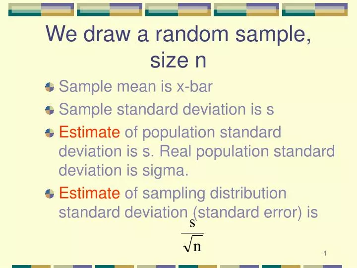
We draw a random sample, size n. Sample mean is x-bar Sample standard deviation is s Estimate of population standard deviation is s. Real population standard deviation is sigma. Estimate of sampling distribution standard deviation (standard error) is. Consider the range.

E N D
We draw a random sample, size n • Sample mean is x-bar • Sample standard deviation is s • Estimate of population standard deviation is s. Real population standard deviation is sigma. • Estimate of sampling distribution standard deviation (standard error) is
Consider the range • Begin with (x-bar - 2*s/sqrt(n)) • End with (x-bar + 2*s/sqrt(n))
Sampling distribution What is p of each type of sample (1 - 6)? Sample 1 Sample 2 Sample 3 Sample 4 Sample 5 Sample 6
Note • We earlier said population mean ± 2 standard deviations of the sampling distribution (called the standard error of the mean, or just the standard error) will include 95% of the samples. • Now we say that sample mean ± 2 standard errors will include the population mean 95% of the time
In other words • Sample will include thepopulation mean 95% of the time. • Does not depend upon shape or distribution of the population, especially as sample size (n) increases. • When sample is small, we use alternative t distribution rather than the normal distribution
The “t” distribution Fewer cases in the middle Fatter tails
Why the t distribution? • We use the normal distribution when we know the standard deviation of the population. • We use the t distribution when we have to estimate the population standard deviation from the sample. In doing this we lose useful information and the resulting sampling distribution has more cases far from the mean
Why the t distribution? • We loose one piece of information when we calculate the mean. • Consider: 1 2 3 is sample. Now fix mean at 2. What possible values can each case take if mean is 2? • This has a bigger impact when we have a small sample. • How much information is there in a sample? n pieces (n is the sample size)
Lost information • With less information, there is more variability in the sampling distribution. • This means fatter tails and fewer cases in the middle • Look again at the t distribution. This one is for samples of size 10.
The t distribution Fewer cases in the middle Fatter tails
Different t distributions • There is a different t distribution for every sample size. • We label them by the number of degrees of freedom • As the sample size increases (the number of degrees of freedom increases) the t becomes more and more normal in shape
Compare at ± 2 standard errors Sample Size Normal Prob. t Prob. Diff. 10 .0455 .0734 .0279 20 .0455 .0593 .0138 30 .0455 .0546 .0091 40 .0455 .0523 .0068 50 .0455 .0509 .0054 60 .0455 .0500 .0045 100 .0455 .0482 .0027 200 .0455 .0469 .0014 500 .0455 .0460 .0005 1000 .0455 .0458 .0003
With small sample sizes • Mean of sampling distribution is mean of population. Our estimate is xbar • Shape of sampling distribution is t • Standard error is sigma over squareroot of n. Our estimate is
Confidence interval • For large samples, confidence interval for mean is • For small samples, confidence interval for mean is • For large samples, confidence interval for proportions is
Conf. interval & hypothesis test • We have been looking at confidence intervals around means and proportions • An alternative approach is to test a hypothesis. • These two approaches do much the same thing, though we state our conclusions differently
Confidence interval conclusion • The population mean (proportion) is likely (95%) to be within this interval or
Hypothesis-test conclusion • I am confident (95%) that this sample did not come from the hypothesized population. Therefore I reject the hypothesis. • I cannot reject the hypothesis that the sample came from the hypothesized population.
Compare • Reject any hypothesis that was outside the confidence interval (H1) • Fail to reject any hypothesis that was within the confidence interval (H2) H1 H2
Which samples would reject Hypothesis of mean at the blue line? Sampling distribution Sample 1 Sample 2 Sample 3 Sample 4 Sample 5 Sample 6