The Supply Chain

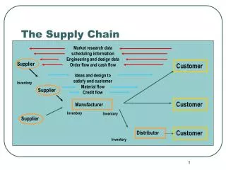
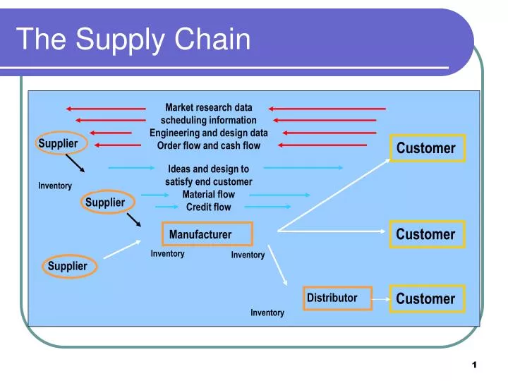
1. Market research data scheduling information Engineering and design data Order flow and cash flow Supplier Customer Ideas and design to satisfy end customer Material flow Credit flow Inventory Supplier Customer Manufacturer Inventory Inventory Supplier Customer Distributor Inventory The Supply Chain

2. Supply Chain Management • Facilities, functions, activities for producing & delivering product or service from supplier to customer • Production planning • Selecting suppliers • Purchasing materials • Identifying facility locations • Managing inventories • Distributing product

3. Transportation Model Given a set of facilities/locations, identify the shipping strategy that will minimize the total costs of distributing the product from the supply nodes to the demand nodes. Supply nodes = sources where units are being sent from Demand nodes = destinations where units are being received

4. Network Of Routes for KPiller Harbors (Sources) Plants (Destinations) $120 Amsterdam (500) Leipzig (400) $130 $62 $41 Nancy(900) $61 $100 Antwerp (700) $40 $110 Liege (200) $90 $102.5 $122 Le Havre (800) Tilburg (500) $42

5. The Transportation Tableau To Supply Leipzig Nancy Liege From Tilburg 120 130 41 62 500 Amsterdam 61 100 40 110 700 Antwerp 102.5 90 122 42 800 Le Havre Demand 400 900 200 500

6. Excel Model • Create a table for the unit shipping costs • Create a table for the shipping quantity from each source to each destination (sink) • Calculate the total shipped from each source • Calculate the total received at each destination • Calculate the total shipping cost for a shipping strategy • Create the spreadsheet model for the problem using the template outlined in TPmodels.xls

7. Solver Constraints for the TP Model • Total shipped from each source <= Supply • Total received at each destination = Demand • Amount shipped from each source to each destination >= 0 • Note: if you are minimizing transportation costs and you do not require the model to satisfy demand, Solver will choose to not ship anything and incur a cost of $0.

8. Balanced Transportation Models • A transportation problem is balanced if Total supply at all of the sources = Total demand at all of the destinations • The KPilller transportation problem is currently balanced with Total Supply = Total Demand = 2000 engines • In this case, all of the units are shipped from the sources (harbors) and all of the destinations (plants) receive their demand

9. Unbalanced Transportation Models • If Total supply at all of the sources > Total demand at all of the destinations, the problem is feasible. There will be unshipped units at some of the source locations though. • (Resolve model with Nancy’s plant demand set equal to 700 engines) • If Total supply at all of the sources < Total demand at all of the destinations, the problem will be infeasible. • (Resolve model with Nancy’s plant demand set equal to 1000 engines)

10. Redefining an Infeasible Unbalanced Transportation Model • If the objective is changed to maximize profit or revenue, the problem can then be solved by changing the demand constraint: • Total received at each destination <= Demand • Note: with the new objective, Solver will choose to ship as much as possible. Not all demand will be satisfied even though the problem is now feasible. To ensure that all destinations receive a reasonable amount of product ,a minimum demand constraint can be added to the current demand constraint for each destination: • Total received at each destination >= Minimum Acceptable Demand

11. Solving an Infeasible Unbalanced Transportation Model • The model needs to be re-balanced in order to identify an optimal shipping strategy when minimizing costs remains the objective • Include an extra source into the model to supply the current shortage or • Set the minimal percent of demand at each destination that must be met to keep customer happy and yet does not result in an overall shortage (e.g. 95% of each plant’s demand) .

12. Balancing a Transportation Model By Adding a New Source • Include an Extra Source to Supply the Current Shortage • Extra capacity needed = Total demand at all destinations – Total supply at all current sources • To create this additional source of supply/capacity, either • Acquire a new facility/harbor and include it in the network design and spreadsheet model’s table structure or • add a Dummy source into the model’s table structure

13. Solving the KPiller Transportation Problem when Nancy wants 1000 engines • In this problem, the total demand exceeds the total supply by 2100 – 2000 = 100 engines • Insert a dummy harbor with a capacity of 100 engines and a unit shipping cost of $0 to each plant. Edit the spreadsheet model and Solver dialog box to include this new imaginary source. • The identified optimal solution will identify how many engines to ship from each harbor to each of the plants. The engines shipped from the dummy harbor are units that will not actually be distributed; these are the amounts that the receiving plants will be short in the eventual distribution.

14. Contracting a new harbor deal when Nancy’s demand is 1000 engines • In this problem, the total demand still exceeds the total supply by 2100 – 2000 = 100 engines • Insert a possible location for a harbor with a capacity of at least 100 engines along with the identified unit shipping costs from this location to each plant. Edit the spreadsheet model and Solver dialog box to include the new harbor warehouse at this location. • The identified optimal solution will identify how many engines to ship from each harbor, including the additional harbor at the new location, to each of the plants so as to minimize total costs

15. Questions to Reflect on…. • How would you use the transportation model to identify whether Hamburg or Gdansk might be a better location for an additional harbor? • What happens when you do not add a new “real location” to the network but use a dummy source which ends up shipping primarily to one destination? What can you do to resolve this problem?

16. Ragsdale Case 3.1 • “Putting the Link in the Supply Chain” • What type of models have we studied in this class to help you analyze this case? Sketch out the layout of the different models that you would need to integrate on a piece of paper. • How would you link the models together?

17. Network Flow Problem Characteristics • There are three types of nodes in network flow models: • Supply • Demand • Transshipment • Transshipment nodes can both send to and receive from other nodes in the network • In transshipment models, negative numbers represent supplies at a node and positive numbers represent demand.

18. Kpiller Transshipment Problem 1 $120 7 Amsterdam (-500) Leipzig (400) $62 $90 6 $61 Nancy(900) 2 Antwerp (-700) $40 $55 $110 5 Liege (200) $90 $122 3 $60 Le Havre (-800) 4 Tilburg (500) $42

19. Defining the Decision Variables For each arc in a network flow model we define a decision variable as: Xij = the amount being shipped (or flowing) from node ito node j For example… X14 = the # of engines shipped from node 1 (Amsterdam) to node 4 (Tilburg) X56 = the # of engines shipped from node 5 (Liege) to node 6 (Nancy) Note: The number of arcs determines the number of variables!

20. Defining the Objective Function Minimize total shipping costs. MIN: 62X14 + 120X17 + 110X24 + 40X25 +61X27 + 42X34 + 122X35 + 90X36 + 60X45 + 55X56 + 90X67

21. Constraints for Network Flow Problems:The Balance-of-Flow Rules For Minimum Cost Network Apply This Balance-of-Flow Flow Problems Where: Rule At Each Node: Total Supply > Total Demand Inflow-Outflow >= Supply or Demand Total Supply < Total Demand Inflow-Outflow <=Supply or Demand Total Supply = Total Demand Inflow-Outflow = Supply or Demand

22. Defining the Constraints • In this illustration: Total Supply = 2000 Total Demand = 2000 • For each node we need a constraint: Inflow - Outflow = Supply or Demand • Constraint for node 1: –X14 – X17 = – 500 This is equivalent to: +X14 + X17 = 500

23. Defining the Constraints • Flow constraints –X14 – X17 = –500 } node 1 -X24 – X25 – X27 = -700 } node 2 -X34 – X35 – X36 = -800 } node 3 + X14 + X24 + X34 – X45 = +500 } node 4 + X25 + X35 + X45 –X56 = +200 } node 5 + X36 + X56 – X67 = +900 } node 6 + X17 + X27 + X67 = +400 } node 7 • Nonnegativity conditions Xij >= 0 for allij

24. Excel’s Sumif Function • The sumif function adds the cells specified by a given condition or criteria • =sumif(range, criteria, sum range) • range are the cells which will be looked at to see if they meet a specified criteria • Criteria specifies the conditions that will allow a row or column to be included in a sum calculation (i.e. = # or label, >0) • Sum range are the cells that are to summed assuming the row or column meets the criteria • Use cautiously as is not always linear

25. Kpiller Transshipment Problem 1 $120 7 Amsterdam (-500) Leipzig (400) $62 500 $90 400 6 $61 Nancy(900) 2 800 Antwerp (-700) $40 $55 100 $110 300 5 Liege (200) $90 $122 3 $60 Le Havre (-800) 4 Tilburg (500) $42