Download
1 / 88
890 likes | 906 Vues
Informed Search and Exploration. Chapter 4 in textbook. Outline. Informed (Heuristic) Search Strategies Heuristic functions How to invent them Local search and optimization Hill climbing, local beam search, genetic algorithms, … Local search in continuous spaces Online search agents.

E N D
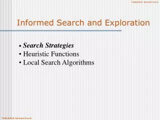
Informed Search and Exploration Chapter 4 in textbook
Outline • Informed (Heuristic) Search Strategies • Heuristic functions • How to invent them • Local search and optimization • Hill climbing, local beam search, genetic algorithms,… • Local search in continuous spaces • Online search agents
Outline • Informed (Heuristic) Search Strategies • Heuristic functions • How to invent them • Local search and optimization • Hill climbing, local beam search, genetic algorithms,… • Local search in continuous spaces • Online search agents
Review: Tree search A strategy is defined by picking the order of node expansion
Best-first search • General approach of informed search: • Best-first search: node is selected for expansion based on an evaluation functionf(n) • Idea: use an evaluation functionf(n)--- estimate of "desirability"for each node • Expand most desirable unexpanded node • Implementation: • fringe is queue sorted in decreasing order of desirability • Special cases: greedy search, A* search
Heuristic function • A key element of evaluation function f(n) • h(n)= estimated cost of the cheapest path from node n to goal node • If n is goal thenh(n)=0
Greedy best-first search • Greedy best-first search expands the node that appears to be closest to goal • Evaluation function f(n) = h(n) (heuristic) = estimate of cost from n to goal
Example • hSLD = straight-line distance from n to Bucharest • hSLD can NOT be computed from the problem description itself • In this example f(n)=h(n) • Expand node that is closest to goal • = Greedy best-first search
Greedy search example • Assume that we want to use greedy search to solve the problem of traveling from Arad to Bucharest. • The initial state=Arad
Greedy search example • The first expansion step produces: • Sibiu, Timisoara and Zerind • Greedy best-first will select Sibiu
Greedy search example • If Sibiu is expanded we get: • Arad, Fagaras, Oradea and Rimnicu Vilcea • Greedy best-first search will select: Fagaras
Greedy search example • If Fagaras is expanded we get: • Sibiu and Bucharest • Goal reached !! • Yet not optimal (see Arad, Sibiu, Rimnicu Vilcea, Pitesti)
Properties of greedy best-first search • Complete?No (cf. DF-search) • Minimizing h(n) can get stuck in loops, e.g. Iasi to Fagaras: Iasi Neamt Iasi Neamt
Properties of greedy best-first search • Complete?No (cf. DF-search) • Time complexity? • Cf. Worst-case DF-search: O(bm) (with m maximum depth of search space) • Good heuristic can give dramatic improvement
Properties of greedy best-first search • Complete?No (cf. DF-search) • Time complexity? O(bm) • Space complexity? O(bm) • keeps all nodes in memory
Properties of greedy best-first search • Complete?No (cf. DF-search) • Time complexity? O(bm) • Space complexity? O(bm) • Optimal?No • Same as DF-search
A* search • Best-known form of best-first search • Idea: avoid expanding paths that are already expensive. • Evaluation function f(n)=g(n) + h(n) • g(n) the cost (so far) to reach the node n. • h(n) estimated cost to get from the node n to the goal • f(n) estimated total cost of path through n to goal
A* search • A* search uses an admissible heuristic • A heuristic is admissible if it never overestimates the cost to reach the goal • Are optimistic • Formally: 1. h(n) <= h*(n) where h*(n) is the true cost from n 2. h(n) >= 0 so h(G)=0 for any goal G • e.g. hSLD(n) never overestimates the actual road distance Theorem: If h(n) is admissible, A* using TREE-SEARCH is optimal
A* search example • Find Bucharest starting at Arad • f(Arad) = c(Arad,Arad) +h(Arad)=0+366=366
A* search example • Expand Arad and determine f(n) for each node • f(Sibiu)=c(Arad,Sibiu)+h(Sibiu)=140+253=393 • f(Timisoara)=c(Arad,Timisoara)+h(Timisoara)=118+329=447 • f(Zerind)=c(Arad,Zerind)+h(Zerind)=75+374=449 • Best choice is Sibiu
A* search example • Expand Sibiu and determine f(n) for each node • f(Arad)=c(Sibiu,Arad)+h(Arad)=280+366=646 • f(Fagaras)=c(Sibiu,Fagaras)+h(Fagaras)=239+179=415 • f(Oradea)=c(Sibiu,Oradea)+h(Oradea)=291+380=671 • f(Rimnicu Vilcea)=c(Sibiu,Rimnicu Vilcea)+ h(Rimnicu Vilcea)=220+192=413 • Best choice is Rimnicu Vilcea
A* search example • Expand Rimnicu Vilcea and determine f(n) for each node • f(Craiova)=c(Rimnicu Vilcea, Craiova)+h(Craiova)=360+160=526 • f(Pitesti)=c(Rimnicu Vilcea, Pitesti)+h(Pitesti)=317+100=417 • f(Sibiu)=c(Rimnicu Vilcea,Sibiu)+h(Sibiu)=300+253=553 • Best choice is Fagaras
A* search example • Expand Fagaras and determine f(n) for each node • f(Sibiu)=c(Fagaras, Sibiu)+h(Sibiu)=338+253=591 • f(Bucharest)=c(Fagaras,Bucharest)+h(Bucharest)=450+0=450 • Best choice is Pitesti !!!
A* search example • Expand Pitesti and determine f(n) for each node • f(Bucharest)=c(Pitesti,Bucharest)+h(Bucharest)=418+0=418 • Best choice is Bucharest !!! • Optimal solution (only if h(n) is admissable)
Optimality of A*(standard proof) • Suppose some suboptimal goal G2has been generated and is in the fringe. Let n be an unexpanded node in the fringe such that n is on a shortest path to an optimal goal G f(G2 ) = g(G2 ) since h(G2 )=0 > g(G) since G2 is suboptimal > f(n) since h is admissible Since f(G2) > f(n), A* will never select G2 for expansion
BUT …if graph search • Discards new paths (if optimal) to repeated state • Previous proof breaks down • Solution: • Add extra bookkeeping i.e. remove more expensive one of the two paths • Ensure that optimal path to any repeated state is always first followed • Extra requirement on h(n): consistency (monotonicity)
Consistent heuristics • A heuristic is consistent if for every node n, every successor n' of n generated by any action a, h(n) ≤ c(n,a,n') + h(n') • If h is consistent, we have f(n') = g(n') + h(n') = g(n) + c(n,a,n') + h(n') ≥ g(n) + h(n) = f(n) • i.e., f(n) is non-decreasing along any path Theorem:If h(n) is consistent, A* using GRAPH-SEARCH is optimal
Optimality of A*(more useful) • A* expands nodes in order of increasing f value • Contours can be drawn in state space • Uniform-cost search adds circles • F-contours are gradually Added: 1) All nodes with f(n)<C* 2) Some nodes on the goal Contour (f(n)=C*). Contour i has all Nodes with f=fi, where fi < fi+1
Properties of A* search • Completeness: YES • Since bands of increasing f are gradually added • Unless there are infinitely many nodes with f<f(G)
Properties of A* search • Completeness: YES • Time complexity: • Number of nodes expanded is still exponential in the length of the solution
Properties of A* search • Completeness: YES • Time complexity: (Exponential with path length) • Space complexity: • It keeps all generated nodes in memory • Hence space, not time, is the major problem
Properties of A* search • Completeness: YES • Time complexity: (Exponential with path length) • Space complexity: (All nodes are stored) • Optimality: YES---Cannot expand fi+1 until fi is finished • A* expands all nodes with f(n)< C* • A* expands some nodes with f(n)=C* • A* expands no nodes with f(n)>C* Also optimally efficient
Unfortunately, … • 在搜索空间中处于目标等值线以内的结点数量仍然是解长度的指数级 • 非指数级的条件: • 两种变换的方法: 1. 使用A*的变种快速找到非最优解 2. 可以设计更准确但不是严格可采纳的启发式
Memory-bounded heuristic search • Some solutions to A* space problems (maintain completeness and optimality) • Iterative-deepening A* (IDA*) • Here cutoff information is the f-cost (g+h) instead of depth • Recursive best-first search(RBFS) • Recursive algorithm that attempts to mimic standard best-first search with linear space • (simple) Memory-bounded A* ((S)MA*) • Drop the worst leaf node when memory is full
Recursive best-first search • Keeps track of the f-value of the best-alternative path available • If current f-value exceeds this alternative f-value then backtrack to alternative path • Upon backtracking change f-value to the best f-value of its children • Re-expansion of this result is thus still possible
Example for RBFS • Path until Rumnicu Vilcea is already expanded • Above node: f-limit for every recursive call is shown on top • Below node: f(n) • The path is followed until Pitesti which has a f-value worse than the f-limit
Example for RBFS • Unwind recursion and store best f-value for current best leaf Pitesti result, f [best] RBFS(problem, best, min(f_limit, alternative)) • best is now Fagaras; Call RBFS for new best • best value is now 450
Example for RBFS • Unwind recursion and store best f-value for current best leaf Fagaras result, f [best] RBFS(problem, best, min(f_limit, alternative)) • best is now Rimnicu Viclea (again); Call RBFS for new best • Subtree is again expanded • Best alternative subtree is now through Timisoara • Solution is found since because 447 > 417
RBFS evaluation • RBFS is a bit more efficient than IDA* • Still excessive node generation (“mind changes”) • Like A*, optimal if h(n) is admissible • Space complexity is O(bd) • IDA* retains only one single number (the current f-cost limit) • Time complexity difficult to characterize • Depends on accuracy of h(n) and how often best path changes • IDA* and RBFS suffer from using too little memory
(Simplified) Memory-bounded A* • Use all available memory • i.e., expand best leaves until available memory is full • When full, SMA* drops worst leaf node (highest f-value) • Like RFBS, backup forgotten nodes to its parent • What if all leaves have the same f-value? • Same node could be selected for expansion and deletion • SMA* solves this by expanding newest best leaf and deleting oldest worst leaf • SMA* is complete if solution is reachable, optimal if optimal solution is reachable • 从实用的角度,SMA*算法是寻找最优解的最好的通用算法
Learning to search better • All previous algorithms use fixed strategies • Agents can learn to improve their search by exploiting the meta-level state space • Each meta-level state is a internal (computational) state of a program that is searching in the object-level state space • In A* such a state consists of the current search tree • A meta-level learning algorithm learns from experiences (e.g. wrong search steps) at the meta-level
Outline • Informed (Heuristic) Search Strategies • Heuristic functions • How to invent them • Local search and optimization • Hill climbing, local beam search, genetic algorithms,… • Local search in continuous spaces • Online search agents
Heuristic functions E.g., for the 8-puzzle: • Avg. solution cost is about 22 steps (branching factor +/- 3) • Exhaustive search to depth 22: 3.1 x 10¹⁰ states • A good heuristic function can reduce the search process
Heuristic functions E.g., for the 8-puzzle knows two commonly used heuristics • h1 = the number of misplaced tiles • h1(s)=8 • h2 = the sum of the distances of the tiles from their goal positions (manhattan distance) • h2(s)=3+1+2+2+2+3+3+2=18
Heuristic accuracy • Effective branching factor b* • Is the branching factor that a uniform tree of depth d would have in order to contain N+1 nodes • Measure is fairly constant for sufficiently hard problems • Can thus provide a good guide to the heuristic’s overall usefulness • A good value of b* is 1
Heuristic accuracy and dominance • 1200 random problems with solution lengths from 2 to 24 • If h2(n) >= h1(n) for all n (both admissible) then h2 dominates h1 and is better for search
Inventing admissible heuristicsⅠ • Admissible heuristics can be derived from the exact solution cost of a relaxed version of the problem • 8-puzzle: 一个棋子可以从方格A移动到B,如果A与B水平或垂直相邻而且B是空的 • Relaxed 8-puzzle for h1 : a tile can move anywhere As a result, h1(n) gives the shortest solution • Relaxed 8-puzzle for h2 : a tile can move to any adjacent square As a result, h2(n) gives the shortest solution
Inventing admissible heuristics • The optimal solution cost of a relaxed problem is no greater than the optimal solution cost of the real problem E.g., ABSolver found a useful heuristic for the magic cube! • 如果一个可采纳启发式的集合h1,…,hm对问题是可用的,则最好的选择是: h(n)=max{h1(n),…,hm(n)}