Download
1 / 51
560 likes | 856 Vues
System-Level Power/Energy Optimization. Dynamic power management. Variable voltage techniques. Memory optimization techniques Hardware-Software partitioning Instruction-level power optimization Control-data-flow transformations. Variable voltage techniques Dynamic power management

E N D
System-Level Power/Energy Optimization Dynamic power management Variable voltage techniques
Memory optimization techniques Hardware-Software partitioning Instruction-level power optimization Control-data-flow transformations Variable voltage techniques Dynamic power management Interface power minimization Approximate signal processing System-Level Power/Energy Optimization
Variable- Voltage Techniques Software Energy Reduction Techniques for Variable- Voltage Processors
Variable- Voltage Techniques • A processor consumes far less energy running tasks requiring a low supply voltage than it does executing high-performance tasks • Using software to dynamically vary supply voltages • Minimizing energy consumption and accommodating timing constraints
Variable- Voltage Techniques • Tasks with severe real-time constraints can execute at high supply voltages • Tasks with loose time constraints can execute at low supply voltages • Energy consumption integrates power consumption in the time domain
Variable- Voltage Techniques • The energy consumption per clock cycle for a task is where M is the number of gates in the circuit, LCk is the load capacitance of gate gk, SWk is the switching count of gk per clock cycle for the task, and VDD is the supply voltage
Variable- Voltage Techniques • The energy consumption for a task with total number of execution cycles CYtask is: • We can reduce the energy consumption for the task by lowering VDD. However, this step increases the execution time.
Variable- Voltage Techniques • The circuit delay T is • and execution time Ttask is: • where VT is the threshold voltage, and VG (~VDD) is the input-gate voltage. The α factor depends on the carrier velocity saturation and in advanced MOSFETs is about 1.3
Dynamically controlled variable-voltage processors • Employs special instructions for controlling supply voltage • CPU clock is adjusted to the frequency suitable for the present supply voltage • The time and power overhead to change the supply voltage is usually important
Motivational example • Assume a given program’s energy consumptions are 10 nJ/cycle at 2.5 V, 25 nJ/cycle at 4.0 V, and 40 nJ/cycle at 5.0 V • The processor’s corresponding computational speeds are 25 × 106, 40 × 106, and 50 × 106 clock cycles/second • Figure 1 shows three voltage assignments for the given program, which has 1 billion execution cycles
Motivational example – cont. • a) the total energy consumption is 40 J, because the processor uses only a 5.0-V supply voltage • b) given a time constraint of 25 seconds, voltage scheduling with 2.5 V and 5.0 V reduces the energy consumption from 40 J to 32.5 J • c) shows the lower-bound case of this example.
Load capacitances • which are charged and discharged by the tasks • because of them, processing the program with a single voltage that adjusts the execution time to the timing deadline does not always minimize energy consumption
Load capacitances – cont. • The average capacitive load per cycle of taskj is: • where the jth task (taskj) is {Xj, Cj}, Xj is the number of execution cycles of the jth task (1≤ j ≤ N), Cj is the average capacitive load for the jth task, M is the number of gates in the processor, LCk is the load capacitance of a gate gk, and SWkij is the switching count of gk while the ith cycle of taskj executes.
Example • For a given task set {task1, task2}, • a) Voltage schedule with a single voltage 4.0 V • b) The voltage scheduling with 2.5 V and 5.0 V • For both voltage schedules, a processor completes the program’s 1 billion cycles only at the timing constraint • The x-, y-, and z-axes of the graphs indicate the execution cycles, the square of supply voltage, and the capacitive loads. The volume of cubes indicates the energy consumption for processing.
Software techniques • Voltage scheduling for real-time applications is complex for several reasons: • A real-time application consists of two or more tasks. In certain applications, precedence relations exist among tasks • A variable-voltage processor uses only a few discrete voltages (or frequencies) because preparing a lot of discrete voltages makes the test difficult
Software techniques – cont. • The load capacitance is different for each task. It depends on input data and does not remain constant during a task’s execution. • Tasks typically end earlier than they would in worst-case execution cycles. However, the scheduler can’t know the execution cycle of the next executed task before that task executes • The scheduler can’t execute a task until it’s ready for execution—the arrival time
Static voltage scheduling • Task set is statically order-scheduled in advance • the CPU time is assigned to tasks using these algorithms on the assumption that the highest supply voltage is used • Then, the supply voltage is assigned to each task to minimize the total energy consumption • If the task set is order-scheduled successfully, the voltage-scheduler can assign a supply voltage to each task without violation of real-time constraints.
Static voltage scheduling • we target real-time, processor-based systems where the processor: • can vary its supply voltage dynamically and at any clock cycle • uses only one supply voltage at a time • employs only a few discrete voltages • has an adaptive clock scheme that closely tracks the supply voltage
Static voltage scheduling • A real-time task Ji is generally characterized by the following parameters: • ai : Arrival time • Oi : Worst case execution time • di : Deadline time • si : Start time of its execution • ei : Completion time of its execution • Li : The remaining time from completion time to deadline
Static voltage scheduling • We additionally define the following parameters to consider energy consumption of the task: • Xi : Worst case execution cycles • Fi : Clock frequency • Oi, Xi and Fi have the following relation • Vi : Supply voltage
Static voltage scheduling - cont • Ci : Average load capacitance where G is the number of gates in the processor, CLk the load capacitance of a gate gk, Switk the average switching count of gk per cycle • Ei : Worst case energy consumption. Ei, Ci, Xi, and Vi have the following relation:
Static voltage scheduling - cont • Here we can see relation between parameters of a real time task
Modification rule 1 • If there is a time period during which no task is executed, the period is called an idle time • The task set is divided into several subsets by idle times
Modification rule 1 - cont • if there is an idle time between two tasks Ji and Ji+1, they are classified into different subsets • Ji is executed at the end of the subset including Ji, and Ji+1 is executed at the beginning of the subset including Ji+1 • If there is a task Jk belonging to the same subset as Ji such that dk > si+1 , the deadline dk is modified as follows:
Modification rule 2 • A task preempted by another task is divided into several subtasks • These subtasks are treated as different tasks
Modification rule 2 - cont • If task Ji is divided into n tasks the arrival time and deadline of task Jij is defined as follows: Moreover, the worst case execution Xij cycles is given by
Formulation of Static Voltage Scheduling • Given: • the task set modified by the rules mentioned above • Xi, di, and Ci for each tasks • processor mode We try to find the function which minimizes
Formulation of Static Voltage Scheduling – cont. subject to: where defined as follows: By solving the this problem, we can obtain the optimal supply voltage assignment on static voltage scheduling
Dynamic voltage scheduling • extend voltage scheduling to tasks for which it is difficult to predict start or completion times • our target system is a real-time system generally includes both application programs and an operating system to execute those applications • a single-processor system, which uses a variable-voltage processor as a processor core, where the variable-voltage processor can discretely change its supply voltage using special instructions for voltage control
Dynamic voltage scheduling - cont • notation is same as in case Static scheduling • Fi and Vi do not change during the execution of Ji • the supply voltage and clock frequency can change when another task preempts Ji, which resumes after the preemption • The following parameters characterize the variable-voltage processor: • (vj, fj) is the processor mode. When the processor’s supply voltage is vj, its clock frequency is fj. • m = |{(vj, fj)}| is the processor’s mode number • Vmax = max(vj) indicates the largest supply voltage
Dynamic voltage-scheduling algorithm • the scheduler assigns a supply voltage to only the next executed task just before task execution • the scheduler must assign supply voltage so that all tasks executed later will not violate these real-time constraints • time slot for each task • A time slot’s start time is when the task execution started. The end time is the maximum time that can guarantee that all future tasks will not violate these real-time constraints
Dynamic voltage-scheduling algorithm - cont • the scheduler’s main work is to determine the time slot’s length for each task • the scheduler’s remaining work is to assign the minimum voltage to the task so that it can finish within its time slot • Two algorithms determine the length of the time slot: • The SD algorithm assumes every task’s arrival time is known • The DD algorithm assumes every task’s arrival time is unknown
Dynamic voltage-scheduling algorithm - cont • SD and DD algorithms have three main steps: • CPU time allocation. Assign the task set CPU time under the condition that all tasks execute on Vmax and that the execution cycle for each task is the worst case • End-time prediction. Determine the time slot’s end time for the next executed task, considering real-time constraints of all later executed tasks • Start-time assignment. Determine the time slot’s start time. The finished time of the previously executed task dynamically moves the start time; the time slot can be lengthened if the previous task finishes ahead of schedule
Dynamic voltage-scheduling algorithm - cont • the SD algorithm performs steps 1 and 2 statically, and step 3 dynamically • the DD algorithm performs all three steps dynamically
Experimental results • We use the following set of tasks: task set = task1, task2, task3 • The average capacitive loads and the number of execution cycles of these three tasks are {C1, X1} = {50 pF, 50 × 109}, {C2,X2} = {100 pF, 50 × 109} , and {C3, X3} = {150 pF, 50 x 109}
Dynamic scheduling • preemptive real-time system
Dynamic scheduling – cont. We scheduled the order and voltage of tasks using the following methods: • Normal. Assign the maximum supply voltage to all tasks • SD. Use the SD algorithm to dynamically assign each task a supply voltage after statically scheduling the execution order. • DD. Use the DD algorithm to dynamically assign each task a CPU time and supply voltage
Dynamic scheduling – cont. • For each scheduling method, the scheduler scheduled tasks in the order:
Dynamic scheduling – Results • In scenario 1 the energy reduction rate was • 38% for SD • 32% for DD • In scenario 2 the energy reduction rate was • 62% for SD • 32% for DD
Dynamic scheduling – Results From the experimental results, we observe the following: • SD and DD always give better results than the normal case • In SD, looser deadline constraints lead to better energy reduction rates because the scheduler has more time to lower the supply voltage • In contrast to SD, power consumption using the DD scheduler is independent of deadline constraints
Variable- Voltage Techniques Power Optimization of Variable-Voltage Core-Based Systems
Experimental results • we used nine applications • the processor cores are assumed operational at the dynamically variable [0.8, 3.3]-V supply voltage • scheduling six different sets of applications and timing constraints on a number of hardware configurations • Each application set was defined using a set of K tasks (K= 10….50) • Each task encompasses one execution of an application