Download
1 / 26
260 likes | 264 Vues
This lecture focuses on evaluating proxy-reconstructed changes within a dynamical framework to advance our understanding of climate dynamics. Topics include choosing a model, the default model for climate variability, and examining climate beasts in the proxy record using this framework.

E N D
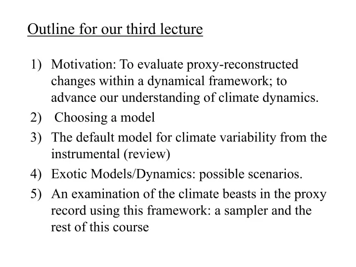
Outline for our third lecture • Motivation: To evaluate proxy-reconstructed changes within a dynamical framework; to advance our understanding of climate dynamics. • Choosing a model • The default model for climate variability from the instrumental (review) • Exotic Models/Dynamics: possible scenarios. 5) An examination of the climate beasts in the proxy record using this framework: a sampler and the rest of this course
1. Motivation • Vision: To evaluate proxy-reconstructed changes within a dynamical framework. • Goal:Establish framework for when changes in circulation matters: WHICH MEANS when do we have to invoke a change (style or magnitude) in the basic circulation regimes, in order to reconcile dynamics with a particular proxy? Can we use current dynamics/understanding of dynamics to explain a proxy? Or Do the proxies compel us to invoke a change in circulation (style or magnitude). • Both improve our understanding of climate history; Only the latter advances the understanding of climate dynamics.
2. Choosing a model:So you have your instrumental or proxy record. How do you understand what it is trying to tell you? • Choose a default model, show the data is inconsistent with it. • Issues to think about: Change in mean vs. change in variability – tricky thing with proxies – tend to reflect extremes, which doesn’t help! • Identify/dream-up scenarios consistent with data - Identify sign and amplitude • Test with a) models b) data. Can this be done?? • Are the data and/or models adequate to truly falsify a hypothesis? A recipe for choosing a “model”
3. The default model for climate variability: A review of lectures 1 &2 • In the midlatitudes, climate variability is due to storm-track dynamics that are intrinsic to the atmosphere • The patterns of climate variability (the ‘modes’) are colocated with the jets, which are determined by gross boundary conditions (e.g., rotation rate, orography, gross land-sea contrasts, etc). • The dynamical time scale associated with these modes is ~ 5 days, and is set by the interactions between the storms and the jets that form them.
Where does variability come from? * Storms owe their existence to the jets. * Over their life cycle, storms both take and give momentum to the jet Storm Decay Storm Growth A “Pattern” is the expression the changes in the jets due to storms.
Examples from the modern climate The NAO The PNA The PDO 0 0.1 0.2 0.3 0.4 0.5 Frequency (/yr) Frequency (/yr)
Where does the memory come from? • The redness of spectrum (presence of enhanced decadal variability is guaranteed because of the interaction with the thermodynamic ocean (time scale 6-12 months. 2) The amplitude of the spectrum and the spatial pattern can be nudged by changes in geometry • e.g., ice sheets, continent configuration, orography, sea ice, sea level, insolation gradient/CO2. 3) On decadal and longer time scales, the memory for reddening may come from other physics: e.g., • 10 years: gyre circulations, arctic sea ice, • 100 years: intermediate water masses; ice streams • 1000 years: ice sheets, deep oceans
The ENSO Mode The modes of the coupled atmosphere-ocean system are found by linearizing the atmosphere and ocean equations about the observed mean state: where is the vector of state variables (SST, 3-D flow fields, thermocline depth, etc) and B is the cyclostationary (due to the mean fields) dynamical matrix. Solving (1), we have (2) where the propagator matrix R is defined using data. Hence, (3) Thus, the yearly propagator is . (4) Thompson and Battisti 2000
The ENSO Mode (cont) • The eigen (Floquet) analysis of Ryear are the true thermo-dynamic modes of the coupled atmosphere system. • The eigenvalues of Ryear yield the frequency and growth rate of the modes, with structures given by the eigenvectors. • The leading (least damped) mode is the ENSO mode, so ENSO is a true model of the coupled atmosphere/ocean system • . The ENSO mode: • Has a rich frequency structure, but a strong spectral peak at 3-4 years, and ‘e-folding’ decay time of two years (cf, the leading “patterns” of stormtrack variability with intrinsic time scales of storm/mean flow interaction (5 days) and reddening due to thermodynamic interaction with the ocean (6-12 months) • ENSO requires a mean state with a strong east-west temperature gradient. Spectrum of the pure ENSO mode
The ENSO mode and Observations • The ENSO mode shares many features of the observed (composite) ENSO cycle: • Bjerknes’ “local” atmosphere/ocean feedbacks in equatorial zone. • A buildup of warm water in the equatorial wave guide that precedes the warming in the eastern Pacific Ocean (ie, the warm phase of ENSO) • The spatio-temporal evolution of ocean heat content (via adiabatic dynamics) throughout the onset, growth and decay of a warm event. e.g., Kessler 1990; Bigg and Blundell 1992; Mantua and Battisti 1994; Wakata and Sarachik 1991; Rosati et al. 1995; Schneider et al. 1995. • The ENSO mode is also consistent with the following observations: • ENSO is peaks at the end of the calendar year because of the annual cycle in the background state of the coupled system. • El Nino events (warm phase of ENSO) last about one year. • The Indian Ocean does not support ENSO variability (homogeneous basic state).
ENSO as a linear, stochastic system 1st EOF from Model 1st EOF from Data Observed Model Results from a linear coupled atmosphere-ocean model forced by white noise -- reproduces essentially all the ‘robust observations’
4. Exotic Models/Dynamics • Impulsive forcing (volcano, ice sheet disintegrating (Heinrich melt-water pulse) • echo of forcing around the globe, but no change in dynamical regime, or new dynamic regime? • new dynamics/circulation regime • A switch between two different dynamical states (i.e., stadial/interstadial)????? • stochastic resonance. • Internal dynamical cycles • ENSO, Quasi-Biennial Oscillation (a tropical stratospheric phenomenon w/ energy at 2-3 years), etc • “Intraseasonal Oscillation” or “Madden Julian Oscillation” • influence on hurricane tracks and Indian monsoonal rainfall • Bond cycles?? • Slip-stick cycles in ice sheets • Exotic physics
5. The climate beasts in the proxy record: do they justify an exotic dynamical model? • Tropical Atlantic Variability (TAV) • Atlantic Multidecadal Oscillation (AMO) • Little Ice Age • Millennial variability in the last glacial period • Antarctica • Greenland & Dansaard/Oescheger Events • Bipolar See-saw • Heinrich Events and 8.2 kyr event • Bond Cycles • Milankovitch (ice age cycles)
Ice core d18O records Antarctica Greenland 0ka 90ka Time Best dated, (and cross dated) records available d18O a more direct reflection of climate than other proxies
Case for the prosecution I: “The clock” Rahmstorf (2003) • Abrupt events happen paced by a ~1500-yr cycle. • GISP2 record suggests a 23 cycle phase memory!
-80kyr -20kyr Time
The GISP2 record is clearly different from the default picture of climate variability.
Assymetry in GISP2 cannot be explained by the default picture…
Is there a Relationship between Antarctica and Greenland? One possibility: Byrd lagging behind -1 x GISP2 by 400 years Another possibility: Byrd leading - GISP2 dt by 200 years
Cross spectrum between GISP2 and Byrd - frequency by frequency what is the correlation between the records and it is significant? 0 0.1 0.5 1.0 Frequency (=10,000 yrs) (=2000 yrs) (=1000 years) Large, long excursions are clearly connected between hemispheres, It is not clear that that abrupt D/O events are…
Low High Low jet Storm High Storms owe their existence to the jets. Over the life cycle of the storm they both take and give momentum to the jet Low Low The “Patterns” are expression the changes in the jets due to storms High High