Download
1 / 53
580 likes | 826 Vues
Overview of Rough Sets. Rough Sets (Theoretical Aspects of Reasoning about Data) by Zdzislaw Pawlak. Contents. Introduction Basic concepts of Rough Sets information system equivalence relation / equivalence class / indiscernibility relation

E N D
Overview of Rough Sets Rough Sets (Theoretical Aspects of Reasoning about Data) by Zdzislaw Pawlak
Contents • Introduction • Basic concepts of Rough Sets • information system • equivalence relation / equivalence class / indiscernibility relation • set approximation (Lower & Upper Approximations) • accuracy of Approximation • extension of the definition of approximation of sets • dispensable & indispensable • reducts and core • dispensable & indispensable attributes • independent • relative reduct & relative core • dependency in knowledge • partial dependency of attribute (knowledge) • significance of attributes • discernibility Matrix • Example • decision Table • dissimilarity Analysis
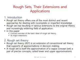
Introduction • Rough Set theory • by Zdzislaw Pawlak in the early 1980’s • use : AI, information processing, data mining, KDD etc. ex) feature selection, feature extraction, data reduction, decision rule generation and pattern extraction (association rules) etc. • theory for dealing with information with uncertainties. reasoning from imprecision data. more specifically, discovering relationships in data. • The idea of the rough set consists of the approximation of a set(X) by a pair of sets, called the low and the upper approximation of this set(X)
Information System • Knowledge Representation System ( KR-system , KRS ) • Information systems • I = < U, Ω> • a finite set U of objects , U={x1, x2, .., xn} ( universe ) • a finite set Ω of attributes , Ω = {q1, q2, .., qm} ={ C, d} • C : set of condition attribute • d : decision attribute • ex) I = < U, {a, c, d}>
Equivalence Relation • An equivalence relation R on a set U is defined as i.e. a collection R of ordered pairs of elements of U, satisfying certain properties. 1. Reflexive: xRx for all x in U , 2. Symmetric: xRy implies yRx for all x, y in U 3. Transitive: xRy and yRz imply xRz for all x, y, z in U
Equivalence Class • R : any subset of attributes( ) • If R is an equivalence relation over U, then U/R is the family of all equivalence classes of R • : equivalence class in R containing an element ex) an subset of attribute ‘R1={a}’ is equivalence relation the family of all equivalence classes of {a} : U/ R1 ={{ 1, 2, 6}{3, 4}{5, 7}} equivalence class : ※A family of equivalence relation over U will be call a knowledge base over U
Indiscernibility relation • If and , then is also an equivalence relation, ( IND(R) ) and will be called an indiscernibility relation over R ※ : intersection of all equivalence relations belonging to R • equivalence class of the equivalence relation IND(R) : • U/IND(R) : the family of all equivalence classes of IND(R) ex) an subset of attribute ‘R={a, c}’ the family of all equivalence classes of {a} : U/{a}={{ 1, 2, 6}{3, 4}{5, 7}} the family of all equivalence classes of {b} : U/{c}={{ 2}{3, 4}{5, 6, 7}{1}} the family of all equivalence classes of IND(R) : U/IND(R) ={{2}{6}{1} {3,4}{5,7}}=U/{a,c}
I = <U, Ω> = <U, {a, c}> Uis a set (called the universe) Ω is an equivalence relation on U(called an indiscernibility relation). • U is partitioned by Ω into equivalence classes, elements within an equivalence class are indistinguishable in I. • An equivalence relation induces a partitioning of the universe. • The partitions can be used to build new subsets of the universe. ※ equivalence classes of IND(R) are called basic categories (concepts) of knowledge R ※ even union of R-basic categories will be called R-category
Set Approximation • GivenI = <U, Ω> • Let and R : equivalence relation • We can approximate X using only the information contained in R by constructing the R-lower( ) and R-upper( ) approximations of X, where or • X is R-definable (or crisp) if and only if ( i.e X is the union of some R-basic categories, called R-definable set, R-exact set) • X is R-undefinable (rough) with respect to R if and only if ( called R-inexact, R-rough)
U U U/R R : subset ofattributes U/R setX set X ∴ X is R-definable • R-positive region of X : • R-borderline region of X : • R-negative region of X : ∴ X is R-rough (undefinable)
EX) I = <U, Ω>, let R={a, c} , X={x | d(x) = yes}={1, 4, 6} ► approximate set Xusing only the information contained in R the family of all equivalence classes of IND(R) : U/IND(R) = U/R = {{1}{ 2}{6} {3,4}{5,7}} R-lower approximations of X : R-lower approximations of X : ※The set X is R-rough since the boundary region is not empty
{x2, x5,x7} {x3,x4} yes {x1,x6} yes/no no Lower & Upper Approximations
Accuracy of Approximation • accuracy measure αR(X) : the degree of completeness of our knowledge R about the set X • If ,the R-borderline region of X is empty and the set Xis R-definable(i.e X iscrisp with respect to R). • If ,the set X has some non-empty R-borderline region and X is R-undefinable (i.e X is rough with respect to R). ex) let R={a, c} , X={x | d(x) = yes}={1, 4, 6}
R-roughness of X : the degree of incompleteness of knowledge R about the set X ex) let R={a, c} , X={x | d(x) = yes}={1, 4, 6} Y={x | d(x) = no}={2, 3, 6, 7} U/IND(R) = U/R = {{1}{ 2}{6} {3,4}{5,7}}
Extension of the definition of approximation of sets • F={X1, X2, ..., Xn} : a family of non-empty sets and => R-lower approximation of the family F : R-upper approximation of the family F : ex) R={a, c} F={X, Y}={{1,4,6}{2,3,5,7}} , X={x | d(x) = yes}, Y={x | d(x) = no} U/IND(R) = U/R = {{1}{ 2}{6} {3,4}{5,7}}
the accuracy of approximation of F : the percentage of possible correct decisions when classifying objects employing the knowledge R • the quality of approximation of F : the percentage of objects which can be correctly classified to classes of F employing the knowledge R ex) R={a, c} F={X, Y}={{1,4,6}{2,3,6,7}} , X={x | d(x) = yes}, Y={x | d(x) = no}
Dispensable & Indispensable • Let R be a family of equivalence relations • let • if IND(R) = IND(R-{a}), then a is dispensable in R • if IND(R) ≠IND(R-{a}), then a is indispensable in R • the family R is independent if each is indispensable in R ; otherwise R is dependent ex) R={a, c} U/{a}={{ 1, 2, 6}{3, 4}{5, 7}} U/{b}={{ 2}{3, 4}{5, 6, 7}{1}} U/IND(R) ={{1}{ 2}{6} {3,4}{5,7}}=U/{a,b} ∴ a, b : indispensable in R ∴ R is independent (∵ U/IR ≠ U/{b}, U/IR ≠ U/{a})
Core & Reduct • the set of all indispensable relation in R => the core of R , ( CORE(R) ) • is a reduct of R if Q is independent and IND(Q) = IND(R) , ( RED(R) ) • ex) a family of equivalence relations R={P, Q, R} • U/P ={{1,4,5}{2,8}{3}{6,7}} • U/Q ={{1,3,5}{6}{2,4,7,8}} • U/R ={{1,5}{6}{2,7,8}{3,4}} • U/{P,Q}={{1,5}{4}{{2,8}{3}{6}{7}} • U/{P,R}={{1,5}{4}{2,8}{3}{6}{7}} • U/{Q,R}={{1,5}{3}{6}{2,7,8}{4}} • U/R={{1,5}{6}{2,8}{3}{4}{7}} U/{P,Q}= U/R =>R is dispensable in R U/{P,R} }= U/R => Q is dispensable in R U/{Q,R} }≠ U/R => P is indispensable in R ∴DORE(R) ={P} ∴RED(R) = {P,Q} and {P,R} (∵ U/{P,Q}≠U/{P} , U/{P,Q}≠U/{Q} U/{P,R}≠U/{P} , U/{P,R}≠U/{R} ) ※ a reduct of knowledge is its essential part. ※ a core is in a certain sense its most important part.
Dispensable & Indispensable Attributes Let R and D be families of equivalence relation over U, if , then the attribute ais dispensable in I , if , then the attribute aisindispensable in I , The R-positive region ofD :
ex) R={a, c} D={d} U/{a}={{ 1, 2, 6}{3, 4}{5, 7}} U/{c}={{ 2}{3, 4}{5, 6, 7}{1}} U/D={{1,4,6}{2,3,5,7}} U/IND(R) ={{1}{ 2}{6} {3,4}{5,7}}=U/{a,c} => the relation ‘a’ is indispensable in R (‘a’ is indispensable attribute) => the relation ‘c’ is indispensable in R (‘c’ is indispensable attribute)
Independent • If every c in R is D-indispensable, then we say that R is D-independent (or R is independent with respect to D) ex) R={a, c} D={d} ∴ R is D-independent ( , )
Relative Reduct & Relative Core • The set of all D-indispensable elementary relation in R will be called the D-core of R, and will be denoted as CORED(R) ※ a core is in a certain sense its most important part. • The set of attributes is called a reduct of R, if C is the D-independent subfamily of R and => C is a reduct of R ( REDD(R) ) ※ a reduct of knowledge is its essential part. ※REDD(R) is the family of all D-reducts of R ex) R={a, c} D={d} CORED(R) ={a, c} REDD(R) ={a, c}
An Example of Reducts & Core • POSR(D)={{1,4,5}{2,3,6}}={1,2,3,4,5,6} • POSR-{a}(D)={{1,4,5}{2,3,6}}={1,2,3,4,5,6} • POSR-{b}(D)={{{1,4,5}{2,3,6}}={1,2,3,4,5,6} • POSR-{c}(D)={{5}}={5} • relation ‘a’, ‘b’ is dispensable • relation ‘c’ is indispensable • => D-core of R =CORED(R)={c} • to find reducts of R={a, b, c} • {a, c} is D-independent and POS{a, c}(D)=POSR(D) • (∵POS{a}(D)={} ≠POS{a, c}(D) • POS{c}(D)={1,4,3,6} ≠POS{a, c}(D) ) • {b, c} is D-independent and POS{b, c}(D)=POSR(D) • => {a, c} {b, c} is the D-reduct of R • POSR-{ab}(D)={{1,4}{3,6}}={1,4,3,6} • POSR-{ac}(D)={{5}}={5} • POSR-{bc}(D)={} U={U1, U2, U3, U4, U5, U6} =let {1,2,3,4,5,6} Ω={headache, Muscle pan, Temp, Flu}={a, b, c, d} condition R={a, b, c}, decision D={d} U/{a}={{1,2,3}{4,5,6}} U/{b}={{1,2,3,4,6}{5}} U/{c}={{1,4}{2,5}{3,6}} U/{a,b}={1,2,3}{4,6}{5}} U/{a,c}={{1}{2}{3}{4}{5}{6}} U/{b,c}={{1,4}{2}{3,6}{5}} U/R={{1}{4}{2}{5}{3}{6}} U/D={{1,4,5}{2,3,6}}
Reduct1 = {Muscle-pain,Temp.} CORE = {Headache,Temp}∩{MusclePain, Temp} = {Temp} Reduct2 = {Headache, Temp.}
Dependency in knowledge • Given knowledge P, Q • U/P={{1,5}{2,8}{3}{4}{6}{7}} • U/Q={{1,5}{2,7,8}{3,4,6}} • If , then Q depends on P (P⇒Q)
Partial Dependency of knowledge • I=<U, Ω> and • Knowledge Q depends in a degree k (0≤k≤1 ) from knowledge P (P⇒k Q) ex) U/Q={{1}{2,7}{3,6}{4}{5,8}} U/P={{1,5}{2,8}{3}{4}{6}{7}} POSP(Q) = {3,4,6,7} the degree of dependency between Q and P : (P⇒0.5 Q ) • If k = 1 we say that Q depends totally on P. • If k < 1 we say that Q depends partially (in a degree k) on P.
significance of attribute ‘b’ : significance of attribute ‘a’ : significance of attribute ‘c’ : Significance of attributes ex) R={a, b, c}, decision D={d} U/{a}={{1,2,3}{4,5,6}} U/{b}={{1,2,3,4,6}{5}} U/{c}={{1,4}{2,5}{3,6}} U/{a,b}={1,2,3}{4,6}{5}} U/{a,c}={{1}{2}{3}{4}{5}{6}} U/{b,c}={{1,4}{2}{3,6}{5}} U/R={{1}{4}{2}{5}{3}{6}} U/D={{1,4,5}{2,3,6}} POSR(D)={{1,4,5}{2,3,6}}={1,2,3,4,5,6} POSR-{a}(D)={{1,4,5}{2,3,6}}={1,2,3,4,5,6} POSR-{b}(D)={{{1,4,5}{2,3,6}}={1,2,3,4,5,6} POSR-{c}(D)={{5}}={5} ∴ the attribute c is most significant, since it most changes the positive region of U/IND(D)
< Decision Table > (a) (b) (c) (d) Discernibility Matrix • Let I = (U, Ω) be a decision table, with U={x1, x2, .., xn} C={a, b, c} : condition attribute set , D={d} : decision attribute set • By a discernibility matrix of I, denoted M(I)={mij}n×n • mijis the set of all the condition attributes that classify objects xi and xjinto different classes. < Discernibility Matrix > - : same equivalence classes of the relation IND(d)
Compute value cores and value reducts from the M(I) • the core can be defined now as the set of all single element entries of the discernibility matrix, • is the reduct of R, if B is the minimal subset of R such that for any nonempty entry c ( ) in M(I) d-reducts : {a, c} {b, c} d-CORE(R)
Proposition 6.2 Each decision table can be uniquely decomposed into two decision tables and such that in and in , where and • compute the dependency between condition and decision attributes • decompose the table into two subtables
decision attribute condition attribute Table 2 • Example 1. Table 3 Table 1 • Table 2 is consistent, Table 3 is totally inconsistent • → All decision rules in Table 2 are consistent • All decision rules in Table 3 are inconsistent
simplification of decision tables : reduction of condition attributes • steps • Computation of reducts of condition attributes which is equivalent to elimination of some column from the decision tables • Elimination of duplicate rows • Elimination of superfluous values of attributes
decision attribute condition attribute • Example 2 remove column c • e-dispensable condition attribute is c. • let R={a, b, c, d}, D={e} • CORED(R) ={a, b, d} • REDD(R) ={a, b, d}
we have to reduce superfluous values of condition attributes in every decision rules → compute the core values • In the 1st decision rules • the core of the family of sets • the core value is
In the 2nd decision rules • the core of the family of sets • the core value is • In the 3rd decision rules • the core of the family of sets • the core value is
In the 4th decision rules • the core of the family of sets • the core value : • In the 5th decision rules • the core of the family of sets • the core value is
In the 6th decision rules • the core of the family of sets • the core value : not exist • In the 7th decision rules • the core of the family of sets • the core value : not exist
to compute value reducts • let’s compute value reducts for the ~ • 1st decision rules of the decision table • 2 value reducts • Intersection of reducts : → core value
2nd decision rules of the decision table • 2 value reducts : • Intersection of reducts : → core value • 3rd decision rules of the decision table • 1 value reduct : • Intersection of reducts : → core value
4th decision rules of the decision table • 1 value reduct : • Intersection of reducts : → core value • 5th decision rules of the decision table • 1 value reduct : • Intersection of reducts : → core value
6th decision rules of the decision table • 2 value reducts : • Intersection of reducts : → core value : not exist
7th decision rules of the decision table • 3 value reducts • Intersection of reducts : → core value : not exist • reducts : = 24 solutions to our problem
One solution Another solution identical enumeration is not essential minimal solution
a b f g c e d 10.4 Pattern Recognition [ Table10 ] : Digits display unit in a calculator assumed to represent a characterization of “hand written” digits ▶ Out task is to find a minimal description of each digit and corresponding decision algorithm.
compute the core attributes [ drop attribute a ] [ drop attribute b ] decision rules are inconsistent Rule1 : b1c1d0e0f0g0 → a0b1c1d0e0f0g0 Rule7 : b1c1d0e0f0g0 → a1b1c1d0e0f0g0
←[drop attribute c] [drop attribute d]→ decision rules are consistent ←[drop attribute e] [drop attribute f]→ decision rules are inconsistent
∴ attribute c, d : dispensable attribute a, b, e, f, g : indispensable the set {a, b, e, f, g} : core sole reducts : {a, b, e, f, g} [drop attribute g] decision rules are inconsistent
compute reduct • all attribute set : {a, b, c, d, e, f, g} • core : {a, b, e, f, g} • reduct : {a, b, e, f, g}
compute the core values of attributes for table11 [Table12 : Removing the attribute a ] [Table13 : Removing the attribute b ] The core value in rule 1 and 4 : a0 The core value in rule 7 and 9 : a1 The core value in rule 5 and 6 : b0 The core value in rule 8 and 9 : b1