Download
1 / 173
1.8k likes | 2.15k Vues
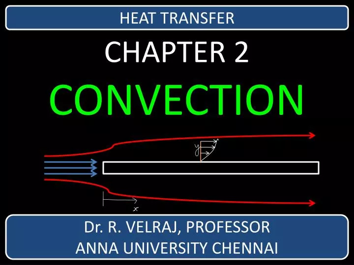
HEAT TRANSFER. CHAPTER 2 CONVECTION. Dr. R. VELRAJ, PROFESSOR ANNA UNIVERSITY CHENNAI. IN THIS SESSION. 1. Introduction to Convection 2. Boundary Layer Concepts. CHAPTER 2 (CONVECTION) – SESSION 1. GOVERNING LAW. Newton’s Law of Cooling Q = h A ( T w – T ∞ ).

E N D
HEAT TRANSFER CHAPTER 2CONVECTION Dr. R. VELRAJ, PROFESSOR ANNA UNIVERSITY CHENNAI
IN THIS SESSION 1. Introduction to Convection2. Boundary Layer Concepts CHAPTER 2 (CONVECTION) – SESSION 1
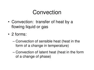
GOVERNING LAW Newton’s Law of CoolingQ = h A (Tw – T∞) h – convective heat transfer coefficient A – surface area over which convection occurs • (Tw – T∞) – temperature potential difference Convection 1
CONCEPT OF BOUNDARY LAYER y TURBULENT REGION LAMINAR REGION TRANSITION x Flow Regimes on a flat plate u∞ u u∞ u FLAT PLATE u = 0 at y = 0 u = u∞ at y = δ Convection 2
FLOW REGIMES ON A FLAT PLATE y Reynolds’ no. x LAMINAR BOUNDARY LAYER Laminar Region (Re < 5 x 10⁵) u∞ u FLAT PLATE τ - Shear stress µ - Dynamic viscosity (proportionality constant) Convection 3
REYNOLDS’ NUMBER Laminar Region ρ Density, kg / m3 u∞ Free Stream Velocity, m / s x Distance from leading edge, m µ Dynamic viscosity, kg / m-s Re < 5 x 10⁵ FLOW OVER FLAT PLATE Re < 2300 FLOW THROUGH PIPE Convection 4
FLOW REGIMES ON A FLAT PLATE TRANSITION Transition Region FLAT PLATE 5 x 10⁵< Re < 106 FLOW OVER FLAT PLATE 2000 < Re < 4000 FLOW THROUGH PIPE Convection 5
FLOW REGIMES ON A FLAT PLATE y x Turbulent Region TURBULENT BOUNDARY LAYER TURBULENT CORE u∞ BUFFER ZONE u LAMINAR SUB LAYER FLAT PLATE Convection 6
FLOW THROUGH TUBE y BOUNDARY LAYER UNIFORM INLET FLOW x Flow Development FULLY DEVELOPED FLOW STARTING LENGTH Convection 7
THERMAL BOUNDARY LAYER y T∞ x TEMPERATURE PROFILE δt TW FLAT PLATE Convection 8
Dimensional Analysis • Reduces the number of independent variables in a problem. • Experimental data can be conveniently presented in terms of dimensionless numbers. • Buckingham’s Pi theorem is used a rule of thumb for determining the dimensionless groups that can be obtained from a set of variables. Convection 9
Buckingham’s Pi theorem Number of independent dimensionless groups that can be formed from a set of ‘m’ variables having ‘n’ basic dimensions is (m – n) Convection 10
QUESTIONS FOR THIS SESSION What is Newton’s Law of Cooling ? Draw the boundary layer for a flow over a flat plate indicating the velocity distribution in the laminar and turbulent flow region. Draw the boundary layer for flow over through tube. Define Buckingham’s π theorem End of Session
Dimensional Analysis • Reduces the number of independent variables in a problem. • Experimental data can be conveniently presented in terms of dimensionless numbers. • Buckingham’s Pi theorem is used a rule of thumb for determining the dimensionless groups that can be obtained from a set of variables. Convection 9
Buckingham’s Pi theorem Number of independent dimensionless groups that can be formed from a set of ‘m’ variables having ‘n’ basic dimensions is (m – n) Convection 10
Dimensional Analysis for Forced Convection Consider a case of fluid flowing across a heated tube Convection 11
Dimensional Analysis for Forced Convection • There are 7 (m) variables and 4 (n) basic dimensions. • 3 (m-n) dimensionless parameters symbolized as π1 ,π2, π3can be formed. • Each dimensionless parameter will be formed by combining a core group of ‘n’ variables with one of the remaining variables not in the core. • The core group will include variables with all of the basic dimensions Convection 12
Dimensional Analysis for Forced Convection Choosing D, ρ, µ and k as the core (arbitrarily), the groups formed is represented as: π1 = DaρbµckdU π2 = DeρfµgkhCp π3 = Djρlµmknh Since these groups are to be dimensionless, the variables are raised to certain exponents (a, b, c,….) Convection 13
Dimensional Analysis for Forced Convection Starting with π1 Equating the sum of exponents of each basic dimension to 0, we get equations for: M 0 = b + c + d L 0 = a – 3b + d + 1 + e T 0 = -d t 0 = -c -3d -1 Convection 14
Dimensional Analysis for Forced Convection Solving these equations, we get: d = 0, c = -1, b = 1, a = 1 giving Similarly for π2 Convection 15
Dimensional Analysis for Forced Convection Equating the sum of exponents M 0 = f + g + I L 0 = e – 3f – g + i + 2 T 0 = -i – 1 t 0 = -g – 3i -2 Solving, we get e = 0, f = 0, g = 1, i = 1 giving Convection 16
Dimensional Analysis for Forced Convection By following a similar procedure, we can obtain The relationship between dimensionless groups can be expressed as F(π1, π2, π3) = 0. Thus, Convection 17
Dimensional Analysis for Forced Convection • Influence of selecting the core variables • Choosing different core variables leads to different dimensionless parameters. • If D, ρ, µ, Cp were chosen, then the π groups obtained would be Re, Pr and St. • St is Stanton number, a non dimensional form of heat transfer coefficient. Convection 18
Dimensional Analysis for FreeConvection Free Convection on a Vertical Plate g T∞ (FLUID) TS (SURFACE) L FLUID PROPERTIES ρ,µ, CP, k, βg Convection 19
Dimensional Analysis for FreeConvection Free Convection on a Vertical Plate In free convection, the variable U is replaced by the variables ΔT, β and g. Convection 20
Dimensional Analysis for FreeConvection Convection 21
Dimensional Analysis for Free Convection Choosing L, ρ, µ and k as the core (arbitrarily), the groups formed is represented as: π1 = LaρbµckdΔT π2 = Leρfµikjβg π3 = LlρmµnkoCp π4 = Lpρqµrksh Convection 22
Dimensional Analysis for Free Convection Following the procedure outlined in last section, we get: π1 = (L2ρ2 k ΔT) / µ2 π2 = (Lµβg) / k π3 = (µCp) / k = Pr (Prandtl number) π4 = (hL) / k = Nu (Nusselt number) Grashof Number Convection 23
Dimensional Analysis FORCEDCONVECTION FREECONVECTION Convection 24
PRANDTL NUMBER Multiplying with ρ in the numerator and denominator, Prair = 0.7 Prwater = 4.5 Prliquid Na = 0.011 Convection 25
PRANDTL NUMBER Pr << 1 Pr >> 1 δh δt δt δh Pr = 1 δt=δh δh = Hydrodynamic thickness δt = Thermal Boundary layer thickness Convection 26
QUESTIONS FOR THIS SESSION What are the dimensionless numbers involved in forced convection and free convection ? Define Prandtl number. List the advantages of using liquid metal as heat transfer fluid. Draw the hydrodynamic and thermal boundary layer (in the same plane) for Pr << 1, Pr >> 1 & Pr = 1. End of Session
What is … Continuity Equation Momentum Equation Energy Equation Convection 27
Laminar – Momentum Equation –Flat Plate y u∞ x dy dx FLAT PLATE Convection 28
Laminar Boundary Layer on a Flat Plate Momentum Equation Assumptions Fluid is incompressible Flow is steady No pressure variations in the direction perpendicular to the plate Viscosity is constant Viscous-shear forces in ‘y’ direction are negligible. Convection 29
Continuity Equation Velocity y x u - Velocity in x direction v - Velocity in y direction Convection 30
Continuity Equation – Laminar – Flat Plate Mass flow Convection 31
Continuity Equation Mass balance Mass balance on the element yields: Or Mass Continuity Equation Convection 32
Momentum Equation – Laminar – Flat Plate Pressure Forces y x p - Pressure Convection 33
Momentum Equation – Laminar – Flat Plate Shear Stresses y x µ - Dynamic viscosity u - Velocity in x direction v - Velocity in y direction Convection 34
Momentum Equation – Laminar – Flat Plate Newton’s 2nd Law • Momentum flux in x direction is the product of mass flow through a particular side of control volume and x component of velocity at that point Convection 35
Momentum Equation – Laminar – Flat Plate Momentum flux Convection 36
Momentum Equation – Laminar – Flat Plate Momentum and Force Analysis Net pressure force Net Viscous-Shear force Convection 37
Momentum Equation – Laminar – Flat Plate Equating the sum of viscous-shear and pressure forces to the net momentum transfer in x direction, making use of continuity relation and neglecting second order differentials: Convection 38
Energy Equation – Assumptions Incompressible steady flow Constant viscosity, thermal conductivity and specific heat. Negligible heat conduction in the direction of flow (x direction). y x u∞ dy dx FLAT PLATE Convection 39
Energy Equation – Laminar – Flat Plate y dy x dx Energy convected in (left face + bottom face) + heat conducted in bottom face + net viscous work done on element Energy convected out in (right face + top face) + heat conducted out from top face Convection 40
Energy Equation – Laminar – Flat Plate Energy Convected y x u - Velocity in x direction v - Velocity in y direction Convection 41
Energy Equation – Laminar – Flat Plate Heat Conducted y x Net Viscous Work u - Velocity in x direction v - Velocity in y direction Convection 42
Energy Equation – Laminar – Flat Plate Net Viscous Work u - Velocity in x direction v - Velocity in y direction Convection 43
Energy Equation – Laminar – Flat Plate Writing energy balance corresponding to the quantities shown in figure, assuming unit depth in the z direction, and neglecting second-order differentials: Convection 44