Download
1 / 33
370 likes | 646 Vues
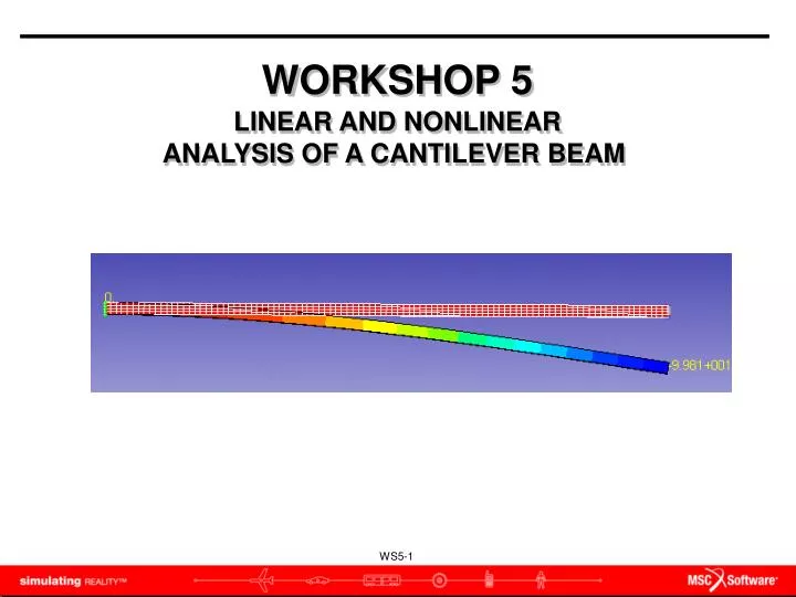
WORKSHOP 5 LINEAR AND NONLINEAR ANALYSIS OF A CANTILEVER BEAM. a. b. Section A-A. Model Description

E N D
WORKSHOP 5 LINEAR AND NONLINEAR ANALYSIS OF A CANTILEVER BEAM
a b Section A-A • Model Description • In this exercise, a cantilever beam is subjected to a static load. The beam is initially analyzed using small deformation theory. However, after reviewing the results, it becomes apparent that small deformation theory is not appropriate for this problem. Subsequently, a large deformation analysis is performed and its results are compared to the small deformation analysis. (Data in next page)
a b Section A-A
Objective • Small vs. large displacement analysis • Linear elastic theory • Required • No Supporting file is required
Suggested Steps for Exercise: • Create simple Cantilever Beam model as illustrated • Use a simple, elastic steel material • Run a linear analysis and look at the results • Run a nonlinear analysis and look at the results • Compare results between linear and nonlinear runs
Step 1. Open a New Database a b Open a new database , Structures Workspace. • Launch SimXpert. • Select Structures.
a b c d f e Step 2. Set Unit Set the units to English. • Select Tools / Options • Select Units Manager. • Click Standard Units. • Select the line containing English Units (in, lb, s…) • Click OK • Click Apply.
Step 3. Create a New Part a Create a New part • On Geometry tab, select Create Part from the Constraint group. • Enter Title as beam. • Click Apply. • Click Cancel. b c d
i b c d j g h f a Step 4. Create a Geometric Surface Create a geometric surface by defining its four vertices. • Click on Filler in theSurface group • Uncheck Using Curves. • Click in the Entities text box. • Select Specify XYZ coordinates from the Pick Filters toolbar. • Enter 0 0 0 then click OK. • Enter 0 0 1, click OK • Enter 0 2 1, click OK. • Enter 0 2 0, click OK then Cancel. • Click OK on the Filler form. • Click Fill on the View Manipulation toolbar. e
d e g c f h i Step 5. Create Mesh Seed a Create Mesh Seed. • In Meshing tab, select Seed. • Click on Curves field. • Select the two curves as the right top graph • Number of Elements: 4 • Click Apply. • Clear the Curve selection by right click icon at the right pf Curves field • Select the two curves as the right bottom graph • Number of Elements: 1 • Click OK b
d c Step 6. Mesh the surface Mesh the Surface. • On the Meshing tab, select Surface in the Automesh group. • Select the Surface in the window. • Choose Mapped in Mesh method option. • Click OK a b a
c e d a Step 7. Sweep Solid Mesh Sweep Solid Mesh. • On the Nodes/Elements tab, select From Shell from the Elements group. • Select the Elements in the window. • Offset:1 • No. of Layers:100 • Click OK. • Click Fill on the View Manipulation toolbar. b
b g d e f h a c Step 8. Delete Shell Elements Delete the plate elements: • Edit / Delete. • Select Elements in the Pick Panel. • Click Advanced… • Highlight Shell • Click All. • Click Done. • Click Yes to Delete unreferenced Nodes. • Click Exit.
a Step 9. Define Material Create the material Steel, with elastic properties. • On the Materials and Properties tab, select Isotropic from the Materials group. • Enter Steel as the Name. • Enter 30E6 as the Young’s Modulus. • Enter 0.3 as the Poisson Ratio. • Click OK.. b c d e
b c d a Step 10. Define Element Properties Create element properties : • On the Materials and Properties tab, select Solid from the 3D Properties group.. • Click the Material text box • Select the material Steel from Model Browser. • Click OK.
Step 11. Assign Element Property to Part Assign property, SOLID_1, to part. • In Model Browser, double click Models \Beam • Click 3D,click right mouse button, Assign Property • Select SOLID_1 • Click OK • Click OK b a c d e
a Step 12. LBC: Fixed Create the fixed Displacement Boundary Conditions. • On the LBC’s tab, select Fixed from the Constraints group • Enter Fixed as the Name. • Pick nodes on the left side • Click OK b c d
600 a Step 13. LBC: Force Create the force load, • On the LBC’s tab, select Force from the Loads group • Enter Tip_Load as the Name. • Pick nodes on the right side • Magnitude: 600 • Direction X,Y,Z :0, -1, 0 • Click OK b c d e f
Step 14. Display LBC Change display mode: Request plotting of Loads/BCs markers on FEM entities. • Click Render On/Off to show LBCs a
Step 15. Create a New Job (Consider geometric nonlinearity) Setup and launch the Analysis. • Right-click FileSet and select Create new Nastran Job. • Enter Nonlinear as the Job Name. • Solution Type: Implicit Nonlinear Analysis (SOL600). • Click OK a b c d
Step 16. Setup Analysis Parameters Setup the Analysis Parameter • Click right mouse button, Simulation / Nonlinear / LoadCases / DefaultLoadCase / Properties • Select SOL600SubcaseNonlinearGeomParameter dialog • Switch Nonlinear Geometric Effects option to Large Displacement/Large Strains • Click Apply • Click Close a b c d e
Step 17. Select Load/BCs Select Load/BCs. • In Model Browser, right click Simulation / Nonlinear / Load Cases / DefaultLoadCase / Load/Boundaries / Select Lbc Set • Select DufaultLbcSet • Click OK.. b c a
Step 18. Run this job Run this job • Open Model Browser, click right mouse button at Nonlinear,select Run. a
Step 19. Attach result file Attach results files, *.t16 • Select File \ Attach Results\ Result Entities… • Choose nonlinear.marc.t16 • Click OK b a c
Step 20. Plot the Deformation Results a c b d e Plot the deformation & stress results. • On the Results tab, select Deformation • Result Cases: select the Increment with Time=1.0 • Result type: Displacement, Translation • Click Display setting tab, change Deformed display scaling to “True :1”. • Choose Update
Step 21. Display Results: Displacement Fringe Display Displacement Fringe • Plot type: Fringe • Result Cases: select the last one • Result Type: Displacement, Translation • Derivation: Y Component • Click Update e c b a d Max. displacement Y= 59.5 in Concern geometric nonlinearity
Step 22. Create a Linear job (No geometric nonlinearity) Setup and launch the Analysis. • Right-click FileSet and select Create new Nastran Job. • Enter Linear as the Job Name. • Solution Type: Linear Analysis (SOL101). • Click OK a b c d
Step 23. Run this job Perform the Analysis • Right click NewJob and select Run. a
Step 24. Attach result file Attach results files, *.t16 • Select File \ Attach Results\ Result Entities… • Choose linear.xdb • Click OK b a c
Step 25. Plot the Deformation Results (No geometric nonlinearity) a c b d e Plot the deformation & stress results. • On the Results tab, select Deformation • Result Cases: SC1: Static Subcase • Result type: Displacement, Translation • Click Display setting tab, change Deformed display scaling to “True :1”. • Choose Update
Step 26. Display Results: Displacement Fringe (No geometric nonlinearity) Display Displacement Fringe • Plot type: Fringe • Result Cases: Select Static Subcase • Result Type: Displacement, Translation • Derivation: Y Component • Click Update e a d b c Linear Case (Don’t consider geometric nonlinearity) Max. displacement Y= 99.8 in
Step 27. Compare with theory in linear case After you apply your graph should look like this The maximum Y deflection of the beam can be taken directly off of the displayed spectrum/range. The largest value should correspond to a magnitude of 99.8, which is in fair agreement with our hand calculation of 100. You may still improve this by remeshing using a finer mesh. (You will be asked to do this after your have ran a nonlinear analysis of present mesh.) Linear beam theory assumes plane section remain plane and the deflection is small relative to length of the beam. As can be clearly seen by this analysis, the deflection is very large and this analysis is in violation of the underlying assumptions used for linear beam theory. These results match the linear hand calculations and also show that the small deformation assumption is not valid and therefore, a non-linear, large deformation analysis needs to be performed. In large deformation analysis, the bending and axial stiffness are coupled. Thus, as the cantilever beam deflects, a portion of the load P puts the beam in tension which tends to stiffen the beam in bending (i.e. “geometric stiffness”). Thus, one would expect to see a much smaller deformation in the large deformation analysis as compared to the small deformation analysis. In our case the deflection is approximately 50% high, it the applied load had been 8000 pounds rather than 6000 our deflection would be approximately 100% high.
Small Deflection Large Deflection -99.8 -59.5 SimXpert/Structure Theory -100.0 -58.59 Compare with these Step 27. Compare Your Results • Compare the results • Finally get the maximum Y deflection from the fringe spectrum/range. Enter that value into the table below. Another interesting post-processing technique is to create an animation by selecting the Animate Results Icon in the Results form. • Also compare the results obtained with both jobs. (Below.)