Download
1 / 17
170 likes | 293 Vues
AMDA-TOPCAT use case. Magnetospheric regions automatic identification V. Génot – October 2012 – V2 vincent.genot@irap.omp.eu Special thanks to the CDPP team, M. Taylor (TOPCAT) & K. Meziane. Science use case. Based on Jelinek et al., JGR 2012 (paper1) Uses AMDA for the analysis

E N D
AMDA-TOPCAT use case Magnetospheric regions automatic identification V. Génot – October 2012 – V2 vincent.genot@irap.omp.eu Special thanks to the CDPP team, M. Taylor (TOPCAT) & K. Meziane
Science use case • Based on Jelinek et al., JGR 2012 (paper1) • Uses AMDA for the analysis • Uses TOPCAT for visualisations • Uses IVOA SAMP to exchange data between AMDA and TOPCAT Goal : • Reproduce two paper1’s results in a few steps • Identify solar wind / magnetosheah / magnetosphere • Identify bow shock and magnetopause • Explore AMDA/TOPCAT enhanced functionalities • AMDA conditional parameters • TOPCAT weighted density maps • Propose new research perspectives
Magnetospheric region identification in Paper1 All THEMIS data 2007/03/01-2009/10/01 magnetosphere With ACE data shifted to THEMIS A position magnetosheath solar wind
THEMIS A magnetospheric sampling over ~3 years 3dview.cesr.fr THEMIS A orbits from 2007/03/01 to 2009/10/01
Magnetospheric regions-- only THEMIS A AMDA – TOPCAT analysis In both cases, the bin/contour represents the number of events Jelinek et al., JGR 2012
Magnetospheric regions rB magnetosphere rB=10rn magnetosheath rB=4-rn solar wind = rn • rB>4-rn • rB<10rn Condition from the plot above : Magnetosheath region
Bow shock and magnetopause identification AMDA – TOPCAT analysis In both case, each bin represents the probability (<1) for this location to be in the magnetosheath In TOPCAT this is automatically computed from the flag_msh values Jelinek et al., JGR 2012
Step by step AMDA–TOPCAT analysis Magnetospheric region identification • define rB and rn in AMDA (create new parameters, see slide for exact definition) • time delay between ACE and THEMIS A is taken constant • for instance : shift(param,4000) shifts ACE data from 4000s forward • here : param=BACE or nACE • a better approach would use (see plot) : T=|XACE-XTHEMIS_A|/VSW • a much better approach would use an iterative algorithm to compute T • for instance see http://cdpp-amda.cesr.fr/DDHTML/HELP/delay.html • launch TOPCAT ; it automatically opens a SAMP hub • in AMDA : click the « interoperability » and open a SAMP connection • download rB and rn on 2007/03/01 – 2009/10/01 at 60s resolution (all in one file) • in AMDA : in the « Download Results » window choose « Send to TOPCAT » • the table is automatically loaded in TOPCAT • choose « density map » (2D histogram) : rB function of rn • adjust binning and plotting range as necessary (0-8 for rn, 0-22 for rB) • do not worry about NaN values !
Step by step AMDA–TOPCAT analysis Bow shock and magnetopause identification Use of AMDA conditional parameters • define the solar wind ram pressure pSW shifted to THEMIS A • time delay may be taken as 4000s as before • pSW=1.67e-6nACEVACE^2 • produce a time table T1 when the pSW values are in a restricted band (ex: pSW<4) • define a new (conditional) parameter : flag_msh • flag_msh=1 if rB>4-rn and rB<10rn (see plot), else 0 (for solar wind and magnetosphere) • download XTHA, sqrt(YTHA^2+ZTHA^2), flag_msh at 3600 s resolution (all in one file) for the above T1 time table Transfer via SAMP (same procedure as before) • the table is loaded into TOPCAT • choose « density map » (2D histogram) : • sqrt(Y^2+Z^2) function of X weighted by flag_msh • adjust binning as necessary
Parameter definition in AMDA r_n = n_i_tha/shiftT_(sw(0),4000) r_b = bs_tha(3)/shiftT_(imf(3),4000) p_sw = shiftT_(sw(0)*sw(1)*sw(1),4000)*1.67e-6 flag_msh = (n_i_tha/shiftT_(sw(0),4000)+bs_tha(3)/shiftT_(imf(3),4000) > 4.) & (bs_tha(3)/shiftT_(imf(3),4000) - 10.*n_i_tha/shiftT_(sw(0),4000) <0.) flag_msh value is either 1 (THEMIS A is in the magnetosheath) or 0
Time delay between ACE and THEMIS A 3dview.cesr.fr It is computed along the XGSE direction : T=|XACE-XTHEMIS_A|/VSW
Time delay T=|XACE-XTHEMIS_A|/VSW Here the delay T is almost constant (2400) so r_b is bs_tha(3)/shiftT_(imf(3),2400) r_b T=2400 r_b
Time delay T=|XACE-XTHEMIS_A|/VSW Here the delay T varies much more, a « banded » delay could be adopted (not implemented here) with conditional parameters : bs_tha(3)/shiftT_(imf(3),2400) or bs_tha(3)/shiftT_(imf(3),3200) or bs_tha(3)/shiftT_(imf(3),4000) r_b r_b In AMDA a conditional parameter P is such that P=1 if P is true Ex: C=A*(T<3600)+B*(T>3600) is equal to either A or B depending on the value of T T=3200 T=4000 T=2400
Perspectives • Refine analysis with smaller ram pressure domains • Extend to larger time intervals, and other S/C (all THEMIS, CLUSTER, …) • Extend to magnetosphere and solar wind region determinations • Use this procedure to deduce bow shock and magnetopause models • Tool enhancements • TOPCAT • Bin value on mouse over • Over plot of contours and user defined lines on density maps • AMDA • Delay procedure (continuous instead of constant or « banded »)