Download
1 / 31
310 likes | 443 Vues
Running Time Performance analysis. Techniques until now: Experimental Cost models counting execution of operations or lines of code. under some assumptions only some operations count cost of each operation = 1 time unit Tilde notation: T(n) ~ (5/3)n 2 Today: Θ- notation

E N D
Lecture 4 Running Time Performance analysis Techniques until now: • Experimental • Cost models • counting execution of operations or lines of code. • under some assumptions • only some operations count • cost of each operation = 1 time unit • Tilde notation: T(n) ~ (5/3)n2 Today: • Θ-notation • Examples: insertionSort & binarySearch
Lecture 4 InsertionSort – Pseudocode • Algorithm (in pseudocode) • for (j = 1; j<A.length; j++) { • //shift A[j] into the sorted A[0..j-1] • i=j-1 • while i>=0 and A[i]>A[i+1] { • swap A[i], A[i+1] • i=i-1 • }} • return A
Lecture 4 Worst Case cost no of times • for (j = 1; j<A.length; j++) { 1 n • //shift A[j] into the sorted A[0..j-1] • i=j-1 1 n-1 • while i>=0 and A[i]>A[i+1] { 1 2+…+n • swap A[i], A[i+1] 1 1+…+(n-1) • i=i-1 1 1+…+(n-1) • }} • return A 1 1 In the worst case the array is in reverse sorted order. T(n) = n + n-1 + Sumx=2..n(x) + 2Sumx=1..n-1(x-1) + 1 = n + n-1 + (n(n+1)/2 - 1) + 2n(n-1)/2 + 1 = (3/2)n2 + (3/2)n - 1 We also saw best- and average-case
Lecture 4 How fast is T(n) = (3/2)n2 + (3/2)n - 1 ? Fast computer vs. Slow computer
Lecture 4 T1(n) = (3/2)n2 + (3/2)n - 1 T2(n) = (3/2)n - 1 Fast Computer vs. Smart Programmer
Lecture 4 T1(n) = (3/2)n2 + (3/2)n - 1 T2(n) = (3/2)n - 1 Fast Computer vs Smart Programmer (rematch!)
Lecture 4 A smart programmer with a better algorithm always beats a fast computer with a worst algorithm for sufficiently large inputs.
Lecture 4 At large enough input sizes only the rate of growth of an algorithm’s running time matters. • That’s why we dropped the lower-order terms with the tilde notation: • When T(n) = (3/2)n2 + (3/2)n -1 • we write: T(n) ~ (3/2)n2 • However: to calculate (3/2)n2 we need to first calculate (3/2)n2 + (3/2)n -1 • It is not possible to calculate the coefficient 3/2 without the complete polynomials.
Lecture 4 Simpler approach It turns out that even the coefficient of the highest order term of polynomials is not all that important for large enough inputs. This leads us to Asymptotic running time: T(n) = (3/2)n2 + (3/2)n - 1 = Θ(n2) • We ignore everything except for the most significant growth function • Even with such a simplification, we can compare algorithms to discover the best ones • Sometimes constants matter in the real-world performance of algorithms, but this is rare.
Lecture 4 Important Growth Functions From better to worse: Function fName • 1 constant • log n logarithmic • n linear • n.log n • n2 quadratic • n3 cubic • … • 2n exponential • ...
Lecture 4 Important Growth Functions From better to worse: Function f Name • 1 constant • log n logarithmic • n linear • n.log n • n2 quadratic • n3 cubic • … • 2n exponential • ... The first 4 are practically fast (most commercial programs run in such Θ-time) Anything less than exponential is theoretically fast (P vs NP)
Lecture 4 Important Growth Functions From better to worse: Function fName Problem size solved in mins (today) • 1 constant any • log n logarithmic any • n linear billions • n.log n hundreds of millions • n2 quadratic tens of thousands • n3 cubic thousands • … • 2n exponential 100 • ...
Lecture 4 Growth Functions From better to worse: Function f Name Example code of Θ(f): • 1 constant swapA[i], A[j] • log n logarithmicj=n; while(j>0){ …; j=j/2} • n linear for(j=1; j<n; j++){ … } • n.log n [best sorting algorithms] • n2 quadratic for(j=1; j<n; j++){ for(i=1; i<j; i++){ … }} • n3 cubic [3 nested for-loops] • … • 2n exponential [brute-force password breaking tries all combinations]
Lecture 4 Asymptotic Running Time Θ(f(n)) It has usefuloperations: • Θ(n) + Θ(n2) = Θ(n2) • Θ(n) × Θ(n2) = Θ(n3) • Θ(n) × Θ(log n) = Θ(n.log n) • Θ(f(n)) + Θ(g(n)) = Θ(g(n)) if Θ(f(n)) ≤ Θ(g(n)) • Θ(f(n)) ×Θ(g(n)) = Θ(f(n) × g(n)) • If f(n) = Θ(g(n)) and g(n) = Θ(h(n)) then f(n) = Θ(h(n))
Lecture 4 InsertionSort – asymptotic worst-case analysis asymptotic cost (LoC model) • for j = 1 to A.length { • //shift A[j] into the sorted A[0..j-1] • i=j-1 • while i>=0 and A[i]>A[i+1] { • swap A[i], A[i+1] • i=i-1 • }} • return A T(n) =
Lecture 4 InsertionSort – asymptotic worst-case analysis asymptotic cost (LoC model) • for j = 1 to A.length { Θ(n) • //shift A[j] into the sorted A[0..j-1] • i=j-1 Θ(n) • while i>=0 and A[i]>A[i+1] { Θ(n2) • swap A[i], A[i+1] Θ(n2) • i=i-1 Θ(n2) • }} • return A Θ(1) T(n) = Θ(n) + Θ(n) + Θ(n2)+ Θ(n2)+ Θ(n2)+ Θ(1) = Θ(n2)
Lecture 4 More Asymptotic Notation O, Ω • When we are giving exact bounds we write: T(n) = Θ(f(n)) • When we are giving upper bounds we write: Τ(n) ≤Θ(f(n))or alternatively T(n) = Ο(f(n)) • When we are giving lower bounds we write: Τ(n) ≥Θ(f(n))or alternatively T(n) = Ω(f(n))
Lecture 4 Examples Θ, O, Ω • 3n2 . log n + n2 + 4n - 2 = ? • 3n2 . log n + n2 + 4n - 2 = O(n2 . log n) • 3n2 . log n + n2 + 4n - 2 = O(n3) • 3n2 . log n + n2 + 4n - 2 = O(2n) • 3n2 . log n + n2 + 4n - 2 ≠ O(n2)
Lecture 4 Examples Θ, O, Ω • 3n2 . log n + n2 + 4n - 2 = Θ(n2 . log n) • 3n2 . log n + n2 + 4n - 2 = Ω(n2 . log n) • 3n2 . log n + n2 + 4n - 2 = Ω(n2) • 3n2 . log n + n2 + 4n - 2 = Ω(1) • 3n2 . log n + n2 + 4n - 2 ≠ Ω(n3 . log n)
Lecture 4 Examples (comparisons) • Θ(n logn) =?= Θ(n)
Lecture 4 Examples (comparisons) • Θ(n logn) > Θ(n) • Θ(n2 + 3n – 1) =?= Θ(n2)
Lecture 4 Examples (comparisons) • Θ(n logn) > Θ(n) • Θ(n2 + 3n – 1) = Θ(n2)
Lecture 4 Examples (comparisons) • Θ(n log(n)) > Θ(n) • Θ(n2 + 3n – 1) = Θ(n2) • Θ(1) =?= Θ(10) • Θ(5n) =?= Θ(n2) • Θ(n3 + log(n)) =?= Θ(100n3+ log(n)) • Write all of the above in order, writing = or < between them
Lecture 4 Principle • Θbounds are the most precise asymptotic performance bounds we can give • O/Ωboundsmay beimprecise
Lecture 4 One more example: BinarySeach Specification: • Input: array a[0..n-1], integer key • Input property:a is sorted • Output: integer pos • Output property: if key==a[i] then pos==i Trivial? • First binary search published in 1946 • First bug-free binary search published in 1962 • Bug in Java’s Arrays.binarySearch() found in 2006
Lecture 4 BinarySearch – pseudocode • lo = 0, hi = a.length-1 • while(lo <= hi) { • intmid = lo + (hi - lo) / 2 • if(key < a[mid]) then hi = mid - 1 • else if (key > a[mid]) then lo = mid + 1 • else returnmid • } • return -1 Note: here array indices start from 0 and go up to length-1.
Lecture 4 BinarySearch – Loop Invariant • lo = 0, hi = a.length-1 • while(lo <= hi) { • intmid = lo + (hi - lo) / 2 • if(key < a[mid]) then hi = mid - 1 • else if (key > a[mid]) then lo = mid + 1 • else returnmid • } • return -1 Note: here array indices start from 0 and go up to length-1. Invariant: if key in a[0..n-1] then key in a[lo..hi]
Lecture 4 BinarySearch – Asymptotic Running Time Asymptotic cost • lo = 0, hi = a.length-1 • while(lo <= hi) { • intmid = lo + (hi - lo) / 2 • if(key < a[mid]) then hi = mid - 1 • else if (key > a[mid]) then lo = mid + 1 • else returnmid • } • return -1 Note: array indices start from 0 and go up to length-1.
Lecture 4 BinarySearch – Asymptotic Running Time Asymptotic cost • lo = 0, hi = a.length-1 Θ(1) • while(lo <= hi) { Θ(log n) • intmid = lo + (hi - lo) / 2 Θ(log n) • if (key < a[mid]) then hi = mid – 1 Θ(log n) • else if(key > a[mid]) then lo = mid + 1 Θ(log n) • else returnmid Θ(log n) • } • return -1 Θ(1) Note: array indices start from 0 and go up to length-1. T(n) = Θ(log n) When a loop throws away half the input array at each iteration: it will perform Θ(log n) iterations!
Lecture 4 • We will use the Asymptotic Θ-notation from now on because it’s easier to calculate • The book uses the ~ notation (more accurate but similar to Θ) • We will mostly look at the worst case (sometimes the average) • Sometimes we can sacrifice some memory space to improve running time • We will discuss space performance and space/time tradeoff in next lecture • Don’t forget the labs tomorrow, Tuesday and Thursday • see website