Download
1 / 38
380 likes | 706 Vues
Contingency Tables. Contingency Tables as Descriptive Statistical Tools. Structure of contingency tables. Symmetry. Rules. Populations and sub-populations. Grand, Column, and Row percentiles. Simpson’s Paradox. Using tables for inference testing – Chi 2.

E N D
Contingency Tables as Descriptive Statistical Tools • Structure of contingency tables. • Symmetry. • Rules. • Populations and sub-populations. • Grand, Column, and Row percentiles. • Simpson’s Paradox. • Using tables for inference testing – Chi2.
Contingency Tables as Descriptive Statistical Tools One of the most common types of statistical tools, so-called because the two variables in the table are contingent upon one another Also called crosstabs because the two variables cross tabulate (or refer to) a single subject. They can be a descriptive or inferential using the Chi2 statistic (pronounced “k-eye” square). Deceptively simple tool; deceptive because they look easy to interpret but are not! Show a wealth of information about population and subsets of that population
Structure of Contingency Tables The variables are in a rXc structure not just columns Groups of rows and columns are defined by one variable each such as eye and hair colour Individual rows and columns represent the sub categories within each variable - e.g. blue, brown, black etc The number of subcategories define the size of the table – e.g. a 4X4 table would have two variables each with foursub categories as follows…
Anatomy of a 4X4 table Variable #1 Subcategory #1 Variable #2 Subcategory #2 Column totals are for VAR #1 Row totals are for VAR #2 Data values for subjects in cells Grand Total Marginal Totals
Contingency Table Symmetry Tables are symmetrical when there are the same number of sub-category rows and columns – e.g. a 4X4 table Tables are asymmetric when there are dissimilar # of sub-category rows and columns – e.g. a 4X6 table Asymmetric tables are difficult to do inferential testing on so avoid them High level tables that have more than two variables also exist but are complex to analyse
Contingency Table Symmetry A 4X4 Table A 4X6 Table
Table rules for mix of variables If variables have a potential relationship then the dependent variable goes on the ‘Y’ axis If one variable is a population then that variable goes on the ‘Y’ axis If both variables are categorical then it does not matter where each goes
Table Rules Cont… Independence: every subject must have the same chance of being selected. Exclusivity: subjects can fall only into one cell; e.g. cannot use data drawn from multiple responses to a single question (no one eye blue, one eye brown or no eye colour!). Exhaustive: subcategories should include all responses received (i.e. the sum of rows must equal the sum of columns, or no-one can have hair colour without eye colour or vice versa). ●
And for the curious… Rarest combinations: 1. Black hair/green eyes = <1 person in 100 2. Blonde hair/brown eyes = 1.2 people in 100 Commonest combinations: 1. Brown hair/brown eyes = 20% of population 2. Blonde hair/blue eyes = @ 16% of population
And for the curious… Rarest combinations: 1. Black hair/green eyes = <1 person in 100 2. Blonde hair/brown eyes = 1.2 people in 100 Commonest combinations: 1. Brown hair/brown eyes = 20% of population 2. Blonde hair/blue eyes = @ 16% of population
Deriving Useful Information Tables depend on proportional calculations using marginal totals (row and column) to be useful. In reality you are dealing with sub groups of the population. Each row total and column total represents a sub-population. Three proportional (percentile) tables are derived and analysed:
Populations and Sub-populations Population as a whole. Variable #1 Sub-population – Hair across all eye categories. Variable #2 sub-population – Eyes across all hair categories.
200 subjects divided among four categories: yes smoke, no smoke, yes disease, no disease ALL SUBJECTS’ RAW DATA 200 total subjects proportionalised to grand total ALL SUBJECTS’ OVERALL STATUS 200 total subjects proportionalised to row (diseased) total DISEASED’ SMOKING STATUS 200 total subjects proportionalised to column (smoke) total SMOKERS’ DISEASE STATUS
200 subjects divided among four categories: yes smoke, no smoke, yes disease, no disease ? ALL SUBJECTS’ RAW DATA 200 total subjects proportionalised to grand total ALL SUBJECTS’ OVERALL STATUS 200 total subjects proportionalised to row (diseased) total DISEASED’ SMOKING STATUS 200 total subjects proportionalised to column (smoke) total SMOKERS’ DISEASE STATUS
200 subjects divided among four categories: yes smoke, no smoke, yes disease, no disease ? ALL SUBJECTS’ RAW DATA 200 total subjects proportionalised to grand total ALL SUBJECTS’ OVERALL STATUS 200 total subjects proportionalised to row (diseased) total DISEASED’ SMOKING STATUS 200 total subjects proportionalised to column (smoke) total SMOKERS’ DISEASE STATUS
200 subjects divided among four categories: yes smoke, no smoke, yes disease, no disease ? ALL SUBJECTS’ RAW DATA 200 total subjects proportionalised to grand total ALL SUBJECTS’ OVERALL STATUS 200 total subjects proportionalised to row (diseased) total DISEASED’ SMOKING STATUS 200 total subjects proportionalised to column (smoke) total SMOKERS’ DISEASE STATUS
Interpreting Raw Data All 200 subjects are divided up among the four categories: Smoker with disease (n=13) Smoker with no disease (n=37) Non-smoker with disease (n=6) Non-smoker with no disease (n=144) And there are four sub-totals: Not diseased (n=181) Non-smokers (n=150) Diseased (n=19) Smokers (n=50) How do we draw conclusions about the risks of smoking from these data?
Interpreting Grand Total Percentiles All 200 subjects are proportionalised to the grand total. Now: Population who smoked and had heart disease (6.5%) Population who smoked and had no heart disease(18.5%) Population who didn’t smoke and had heart disease (3.0%) Population who didn’t smoke and had no heart disease (72%) Are smoking and disease related? Only 26% of smokers were diseased (6.5%/25%*100). Yet 68% of diseased people were smokers (6.5%/9.5%*100)
Interpreting Column Percentiles All 200 subjects are proportionalised to the column total. Now we are interpreting the data from the perspective of a subset of the sample – a person’s smoking status. Now: Smokerwith disease (26%) Smokerwith no disease (74%) Non-smokerwith disease (4%) Non-smokerwith no disease (96%) Now what do we say? About three quarters of smokers don’t get sick! That’s where you would stop the analysis if you worked for the tobacco companies
Interpreting Row Percentiles All 200 subjects are proportionalised to the row total. Now we are interpreting the data from the perspective of the other subset of the sample – a person’s disease status. Now: Diseasedand smoker (68.4%) Not diseased and smoker (20.4%) Diseasedand non-smoker (31.6%) Not diseased and non-smoker (79.6%) Now what do we say? Sixty-eight percent of people with heart disease also smoke while only about 20% of the sample who were free of heart disease were smokers.
Summary Two main points: 1. The different tables give different perspectives so have to be careful to… Use correct subset interpretation – for example, the row-based percentiles in our analysis were about disease status and not smoking status: 68% of people with heart disease smoke, and not 68% of smokers have heart disease!
Summary 2. Watch proportions and size of sample subsets: Only 50 of 200 smoked and… only 19 of 200 had heart disease and… only 13 of 200 had heart disease and smoked. The effect of so many not being diseased and not smoking can overwhelm the other effects, either masking them or exaggerating them.
Simpson’s Paradox Crops up often when using contingency tables in the social sciences. Refers to the apparent reversal of relationships seen in disaggregated data when it is combined. Product of disproportionality among subsets and lurking variables (note the previous smoker/disease data). An example:
Example of Simpson’s ParadoxResults of two surveys done 20 years apart. In both surveys smoker’s die off rates are higher than non-smokers. But when tables are combined, smokers’ die off rates for the whole period are lower. Why? Because dead smokers tell no tales! Smokers die off considerably faster in the earlier period and there are fewer of them around to be counted in the later one. As well, older people’s mortality is obviously higher.
Using Tables for Inference Testing Test for significant differences or relationships rather than just describing the data. Based on comparing the observedcell values to those that could be expected using probability theory and assuming there are no significant differences or relationships. Stated: The probability of falling into a particular cell is the product of the probability of being in a particular row and the probability of being in a particular column.
Calculating Chi Square The statistic most frequently used in inferring with contingency tables is called the Chi Square statistic, written as chi2 and given by the Greek letter χ. It is based on an expected versus actual values methodology and its formula is:
Calculating Chi Square Translated this says: where the expected cell counts are given by:
An Example Are e coli counts different between two lakes in Muskoka, one with cottages and one without? Collect 200 samples of water from each. Measure e coli concentrations. Is the sample above or below acceptable background limit? How to test this?
Collect Observed values Four hundred samples, 200 from each lake
Calculate Expected Values E.G. 124*200/400 = 62
Calculate Deviation Error Squared (O-E)2 Values for Cells E.G. (43-62)2 = 361
Divide (O-E)2 Values by Expected Values E.G. 361/62 = 5.82
Sum the Squared (O-E)2 /Expected Values Chi2= 5.82 +5.82 +2.61 +2.61 = 16.86 Compare 16.86 to the ‘book’ value. If it is greater than book value, there are significant differences in the table.
Interpreting the Example We observed 43 samples from no cottage lakes above background but expected 62 We observed 81 samples from cottage lakes above background but expected 62 We observed 157 samples from no cottage lakes below background but expected 138 We observed 119 samples from cottage lakes below background but expected 138
Remember. Watch your table manners.