Download
1 / 34
340 likes | 452 Vues
Judy Qiu Assistant Professor & Director, Salsa HPC lab Indiana University School of Informatics and Computing xqiu@indiana.edu - http:// salsahpc.indiana.edu. Analyzing large-scale cheminformatics and chemogenomics datasets through dimension reduction. David J. Wild

E N D
Judy Qiu Assistant Professor & Director, Salsa HPC labIndiana University School of Informatics and Computingxqiu@indiana.edu - http://salsahpc.indiana.edu Analyzing large-scale cheminformatics and chemogenomics datasets through dimension reduction David J. Wild Assistant Professor & Director, Cheminformatics ProgramIndiana University School of Informatics and Computingdjwild@indiana.edu - http://djwild.info Geoffrey C. Fox • Associate Dean of Research and Graduate Studies • Director of Digital Science Center Indiana University School of Informatics and Computinggcfd@indiana.edu - http://salsahpc.indiana.edu
Important Trends • Data Deluge • Cloud Technologies • In all fields of science and throughout life (e.g. web!) • Impacts preservation, access/use, programming model • new commercially supported data center model building on compute grids • eScience Multicore/ Parallel Computing • A spectrum of eScience or eResearch applications (biology, chemistry, physics social science and • humanities …) • Data Analysis • Machine learning • Implies parallel computing important again • Performance from extra cores – not extra clock speed
Integrative chemogenomic tools in Wild group – http://djwild.info SPARQL Query Builder: advancedqueryingof Chem2Bio2RDF data Association Search: finding pathsbetween Chem2BioRDF entitiesranked by literature support Chem2Bio2RDF: networking compound,drug, gene, pathway, disease and side-effectinformation using Semantic Web methods BioLDA: integrating recent literatureusing bioterms and providing path rankingusing LDA and KL divergence ChemoHub: quantitativepredictions of relationship strengthbetween compounds and genes WENDI: exploring biological spacearound new chemical compounds Chemogenomic Explorer: exploringcompound-gene-disease relationshipsin a facet browser Plotviz: high dimensional visualizationof query results in chemical space Collaborators: Ying Ding (SLIS), Judy Qiu (SOIC), Lilly, Pfizer
Navigate Chemical Space David Wild, December 2009. Page 4 http://djwild.info Christopher Lipinski & Andrew Hopkins, Pfizer Global R&D, Navigating chemical space for biology and medicine, Nature, Vol 432, 16 Dec 2004 Measured in terms of physicochemical properties and topological descriptors, therapeutically useful compounds appear to cluster together in galaxies. Are these galaxies are evenly and sparsely distributed? Are most of the chemical universe is “empty” (with no therapeutically interesting compounds)?
Salsa HPC group – http://salsahpc.indiana.edu • Large and high-dimensional data visualization • Chemical space visualization • Cheminformatics visual data mining • Parallel dimension reduction algorithms • Parallel Generative Topographic Mapping (GTM) • Parallel Multidimensional Scaling (MDS) • Interpolated GTM/MDS
Introduction to PlotViz • A tool for visualizing data points • Dimension reduction by GTM and MDS • Browse large and high-dimensional data • Use many open (value-added) data
PlotViz System Overview 3-D Map File SPARQL query Meta data PlotViz Light-weight client DrugBank CTD QSAR PubChem Visualization Algorithms Chem2Bio2RDF Parallel dimension reduction algorithms Aggregated public databases
Dimension Reduction Algorithms • Multidimensional Scaling (MDS) [1] • Given the proximity information among points. • Optimization problem to find mapping in target dimension of the given data based on pairwise proximity information while minimize the objective function. • Objective functions: STRESS (1) or SSTRESS (2) • Only needs pairwise distances ijbetween original points (typically not Euclidean) • dij(X) is Euclidean distance between mapped (3D) points • Generative Topographic Mapping (GTM) [2] • Find optimal K-representations for the given data (in 3D), known as K-cluster problem (NP-hard) • Original algorithm use EM method for optimization • Deterministic Annealing algorithm can be used for finding a global solution • Objective functions is to maximize log-likelihood: [1] I. Borg and P. J. Groenen. Modern Multidimensional Scaling: Theory and Applications. Springer, New York, NY, U.S.A., 2005. [2] C. Bishop, M. Svens´en, and C. Williams. GTM: The generative topographic mapping. Neural computation, 10(1):215–234, 1998.
High Performance Data Visualization.. GTM with interpolation for 2M PubChem data 2M PubChem data is plotted in 3D with GTM interpolation approach. Red points are 100k sampled data and blue points are 4M interpolated points. MDS for 100k PubChem data 100k PubChem data having 166 dimensions are visualized in 3D space. Colors represent 2 clusters separated by their structural proximity. GTM for 930k genes and diseases Genes (green color) and diseases (others) are plotted in 3D space, aiming at finding cause-and-effect relationships. [3] PubChem project, http://pubchem.ncbi.nlm.nih.gov/ Developed parallel MDS and GTM algorithm to visualize large and high-dimensional data Processed 0.1 million PubChem data having 166 dimensions Parallel interpolation can process up to 2M PubChem points
Large scale dimension reduction with GTM/MDS Use 2 methods of dimension reduction: GTM clustering (requires descriptor vectors) and MDS (descriptor vectors or similarity matrix) to map descriptor spaces into 3 dimensions Our descriptor spaces are similarity space (MACCS keys) and SALI space (normalized SALI values used as similarity). Only MDS can work with the SALI space
Multidimensional Scaling (MDS) • Given the proximity information among points. • Optimization problem to find mapping in target dimension of the data based on given pairwise proximity information while minimize the objective function. • Objective functions: STRESS (1) or SSTRESS (2) • Only needs pairwise dissimilarities ijbetween original points • (not necessary to be Euclidean distance) • dij(X) is Euclidean distance between mapped (3D) points
Scaling by MAjorizing a COmplicated Function. (SMACOF) Iterative majorizing algorithm to solve MDS problem. EM-like hill-climbing approach. Decrease STRESS value monotonically. Tend to be trapped in local optima. Computational complexity and memory requirement is O(N2).
Deterministic Annealing (DA) • Simulated Annealing (SA) applies Metropolis algorithm to minimize F by random walk. • Gibbs Distribution at T (computational temperature). • Minimize Free Energy (F) • As T decreases, more structure of problem space is getting revealed. • DA tries to avoid local optima w/o random walking. • DA finds the expected solution which minimize F by calculating exactly or approximately. • DA applied to clustering, GTM, Gaussian Mixtures etc.
GTM vs. MDS GTM MDS (SMACOF) Purpose • Non-linear dimension reduction • Find an optimal configuration in a lower-dimension • Iterative optimization method ObjectiveFunction Maximize Log-Likelihood Minimize STRESS or SSTRESS Complexity O(KN) (K << N) O(N2) Optimization Method EM Iterative Majorization (EM-like) • MDS also soluble by viewing as nonlinear χ2 with iterative linear equation solver
Interpolation Method n in-sample Trained data Training N-n out-of-sample Interpolated MDS/GTM map Interpolation Total N data MDS and GTM are highly memory and time consuming process for large dataset such as millions of data points MDS requires O(N2) and GTM does O(KN) (N is the number of data points and K is the number of latent variables) Training only for sampled data and interpolating for out-of-sample set can improve performance Interpolation is a pleasingly parallel application
Interpolation Method Multidimensional Scaling (MDS) Generative Topographic Mapping (GTM) For n samples (n<N), GTM training requires O(Kn) Training computes the optimal position for K latent variables for n data point Out-of-sample data (N-n points) is mapped based on the trained result (No training process required) Interpolation only require O(N-n) memory and time • Find mapping for a new point based on the pre-mapping result of the sample data (n samples). • For the new input data, find k-NN among those sample data. • Based on the mappings of the k-NN, interpolate the new point. • O(n(N-n)) memory required. • O(n(N-n)) computations
Quality Comparison (Original vs. Interpolation) MDS GTM • Quality comparison between Interpolated result upto 100k based on the sample data (12.5k, 25k, and 50k) and original MDS result w/ 100k. • STRESS: wij = 1 / ∑δij2 Interpolation result (blue) is getting close to the original (read) result as sample size is increasing.
Activity Cliffs in PubChem Bioassays • Selected 22 bioassays based on total compounds tested, number of actives, and type diversity. Generally number of compounds with “real” activity numbers << number of actives (with “outcome” field) • Calculated SALI values (Guha, JCIM 2008, 48(3), 646-658) for all pairs of tested compounds in each assay using MACCS keys and log IC50 or percent inhibition: • Investigated pairs with highest SALI values for each bioassay • Simple SALI maps (heatmaps) • Mapping Bioassay Activity Cliffs in Chemical Space • Use multidimensional scaling and GTM methods to project compounds into 3 dimensions using SALI value as a similarity score • Plot compounds in “3D SALI space”, and color by mean SALI score • Compare with simple coloring with activity in 3D similarity space
Modified SALI for polypharmacology Can we look for small changes in activity that produce large changes in polypharmacology profiles? Uses Chem2Bio2RDF (BMC Bioinformatics, 2010, 11, 255) to establish compound-gene relationships. For this study, we identified 10713 compounds associated with at least one of 305 kinases, all from ChEMBL Modified SALI index uses hamming distance of binary association profiles in place of activity value (here Assoc = 1 if there is an association, else 0): Create projections in chemical space where compounds are colored by the number of kinases they are associated with
X(x) • Deterministic Annealing Clustering (DAC) • F is Free Energy • EM is well known expectation maximization method • p(x) with p(x) =1 • T is annealing temperature varied down from with final value of 1 • Determine cluster centerY(k) by EM method • K (number of clusters) starts at 1 and is incremented by algorithm N data points X(x) in D dimensions space and minimize F by EM General Formula DAC GM GTM DAGTM DAGM
DeterministicAnnealing • Minimum evolving as temperature decreases • Movement at fixed temperature going to local minima if not initialized “correctly F({y}, T) Solve Linear Equations for each temperature Nonlinearity effects mitigated by initializing with solution at previous higher temperature Configuration {y}
Redis coarse resolution with 10 clusters Blue is finer resolution with 30 clusters Clusters find cities in Indiana Distance Scale is Temperature Decrease temperature (distance scale) to discover more clusters Deterministic Annealing Clustering of Indiana Census Data
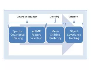
Next Generation Sequencing Pipeline on Cloud MapReduce Pairwise clustering MDS Blast Visualization Plotviz Visualization Plotviz Pairwise Distance Calculation Dissimilarity Matrix N(N-1)/2 values block Pairings Clustering FASTA FileN Sequences 1 2 3 4 • Users submit their jobs to the pipeline and the results will be shown in a visualization tool. • This chart illustrate a hybrid model with MapReduce and MPI. Twister will be an unified solution for the pipeline mode. • The components are services and so is the whole pipeline. • We could research on which stages of pipeline services are suitable for private or commercial Clouds. MPI 5 4
Demos Visualization of pairwise ALU gene alignment byusing Smith Waterman dissimilarity. Metagenomics Visualization of biology dataset Biology Data Bioassay activity/Inactivity classification Visualization of PubChem data by using MDS and GTM PubChem Bioassay active counts
Sample Data MortenAlleso, Frans Van Den Berg, Claus Cornett, Flemming Steen Jorgensen, Bent Halling-Sorensen, Heidi Lopeez De Diego, Lars Hovgaard, JaakkoAaltonen, JukkaRntanen, University of Copenhagen, Solvent Diversity in Polymorph Screening, Journal of Pharmaceutical Sciences, Vol. 97, 2145-2159, 2008 A database of 218 organic solvents with 24 property descriptors The data matrix is analyzed using principal component analysis (PCA) and self-organizing maps (SOMs) methods