Terrain

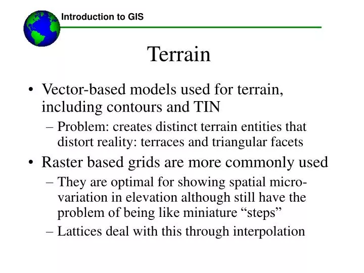
1. Introduction to GIS Terrain • Vector-based models used for terrain, including contours and TIN • Problem: creates distinct terrain entities that distort reality: terraces and triangular facets • Raster based grids are more commonly used • They are optimal for showing spatial micro-variation in elevation although still have the problem of being like miniature “steps” • Lattices deal with this through interpolation

2. Introduction to GIS Weather • Weather station data: Vector, coded with points • Average precipitation surface: Raster interpolation of points • Average precipitation contours: vector lines • Both are interpolations, but one may be more accurate in a given situation • Downside of contours: terrace effect, fewer intervals, more categorical

3. Introduction to GIS Metropolitan Areas • No official administrative boundary for this • Where does one metro area begin and another end? Look at the New York New Jersey area. • For a precise bounding, say for administrative purposes, use vector • Can also include “fuzzy boundaries” • To represent a gradual change from one urban area to another, use raster

4. Introduction to GIS Types of Vector Topology • Arc-node and node topology : the way that line features connect to point features • Polygon topology: the way that neighboring polygons connect and share borders • Route topology: the way that a line feature of one type (e.g. commuter rail line) shares segments with line features of another type (e.g. Amtrack rail line) • Regions topology: the way that polygons overlap (e.g. GIS layers with a time component) or when spatially separate polygons are part of the same feature

5. ------Using GIS-- Introduction to GIS Reclassification with Grids Here we reclass to 3 classes, based on natural breaks

6. ------Using GIS-- Introduction to GIS Reclassification with Grids

7. ------Using GIS-- Introduction to GIS Reclassification with Grids

8. ------Using GIS-- Introduction to GIS Reclassification with Grids

9. Introduction to GIS Raster Data Structuring • Methods for storing raster data in a more computationally and memory efficient way. • Where a raster layer is random noise, this does not work. • Requires repetitive patterns or areas of homogeneity. • The fewer z values, the easier to compress. • Simplest method is cell-by-cell encoding where cell values are stored by row and column number; This is essentially uncompressed. • DEM’s and satellite images generally use this structure because there is typically so much variation.

10. Introduction to GIS Raster Data Structuring • Run-length encoding (RLE): • Compression method that records cell values in groups called “runs.” • It records the starting and ending pixel for a “run” with the same value for a given row, so hundreds of pixels could be recorded with only two values, if they all have the same value and are adjacent. • However, because it measures runs along rows, it is not efficient for two dimensional areas of homogeneity. • RLE can reduce file size by 10:1, depending on data.

11. Introduction to GIS Raster Data Structuring • Runs: • Row 2: 3,4 • Row 3: 2, 8 • Row 4: 4,7 • Row 5: 5,7 • Row 6: 2,6

12. Introduction to GIS Raster Data Structuring • Chain code: • This is a more efficient method for dealing with two-dimensional compression • This defines a homogeneous two-dimensional area using cardinal directions and units movements to define bounding perimeter in relative terms from a known point • For instance, go 2 N, 1 W, 1N, 3 W, 1S….etc.

13. Introduction to GIS Raster Data Structuring • Here, starting from the lower left, the computer would define that coordinate then code 1N, 3E, 1N, 1W, 1N, 2W, 1N, 1E, 1N, 2E etc….. • This would define the perimeter of a homogeneous area. • All must have exactly the same value

14. Introduction to GIS Raster Data Structuring • Block code: • A method that uses square blocks to represent areas of homogeneous values • Each block is encoded only with location of one corner cell and the dimensions; since they are square, only one dimension needs to be given • Uses medial axis transformation technique

15. Introduction to GIS Raster Data Structuring • Quad tree: • Divides a grid into hierarchy of quadrants • Starts with four quadrants; any quadrant that has totally homogeneous cells will not be subdivided further, but is stored as a “lead node” which is coded only with that value and the id of the quadrant. • Any quadrants with more than one value are subdivided again into four more quadrants and again the computer checks for homogeneity. • It keeps on doing this until it has generated all its leaf node or until it gets down to the pixel level • This is known as recursive decomposition • This is good where one part of a grid is very uniform and the rest is heterogeneous.

16. Introduction to GIS Raster Data Structuring • Quad tree: Homogeneous (all one value) Not homogeneous: more than one value within quadrant

17. Introduction to GIS Raster Data Structuring • Quad tree: now we break down those quadrants with non-homogeneous values into four sub quadrants Not homogeneous: more than one value within quadrant

18. Introduction to GIS Raster Data Structuring • Quad tree: and we keep doing this until we’ve come down to the point where there are only homogeneous quadrants, even if those are one cell in dimension Not homogeneous: more than one value within quadrant

19. Introduction to GIS Raster Data Structuring One value (leaf node) Mixed values (non-leaf) • Quad tree:

20. Introduction to GIS Vector Compression Vector data take up a lot of memory, so compression techniques are needed. These are automated techniques for simplifying line segments by removing points, while still preserving geometric accuracy Simplest form is elimination of repetitive characters, like the first character, or coordinate value, of all coordinates along a particular horizontal axis Another is to keep every nth point on a line Yet another is to remove points and estimate functions: Spline function can estimate polynomials

21. Introduction to GIS Vector Compression One of the most common methods is the Douglas-Peucker method Draw a straight line between first and last points in a curved line segment and calculate orthogonal distance from each point to line; those that fall within certain defined distance are removed The new end point of the straight line is then moved to the point with the greatest orthogonal distance and process starts again.

22. Introduction to GIS Vector Compression Douglas-Peucker method

23. Introduction to GIS PLSS • Public Land Survey System is used for partitioning of land • Land is US West and Midwest are divided up into nested hierarchy: • 6x6 mile townships • 36 mile square parcels called sections

24. Introduction to GIS PLSS • Note the nested system

25. Introduction to GIS PLSS • Here are the townships for Washington

26. Introduction to GIS PLSS • BLM is currently developing a Geographic Coordinate Database of PLSS in the west • The database contains lat/long coordinates and descriptive information for section corners and monuments recorded in the PLSS • This is important, because many people’s land ownership in the west is based on this system

27. Introduction to GIS PLSS How it’s been done in the past; survey markers or benchmarks are key

28. Introduction to GIS IDW-How it works • Zij= Zxy /Dp • Z value at location ij is f of Z value at known point xy times the inverse distance raised to a power P. • Z value field: numeric attribute to be interpolated • Power: determines relationship of weighting and distance; where p= 0, no decrease in influence with distance; as p increases distant points becoming less influential in interpolating Z value at a given pixel

29. Introduction to GIS IDW-How it works • What is the best P to use? • It is the P where the Root Mean Squared Prediction Error (RMSPE) is lowest, as in the graph on right • To determine this, we would need a test, or validation data set, showing Z values in x,y locations that are not included in prediction data and then look for discrepancies between actual and predicted values. We keep changing the P value until we get the minimum level of error. Without this, we just guess.

30. Introduction to GIS IDW-How it works • This can be done in ArcGIS using the Geostatistical Wizard • You can look for an optimal P by testing your sample point data against a validation data set • This validation set can be another point layer or a raster layer • Example: we have elevation data points and we generate a DTM. We then validate our newly created DTM against an existing DTM, or against another existing elevation points data set. The computer determine what the optimum P is to minimize our error

31. Introduction to GIS IDW-How it works

32. Introduction to GIS IDW-How it works • There are two IDW method options Variable and fixed radius: • 1. Variable (or nearest neighbor): User defines how many neighbor points are going to be used to define value for each cell • 2. Fixed Radius: User defines a radius within which every point will be used to define the value for each cell

33. Introduction to GIS IDW-How it works • Can also define “Barriers”: User chooses whether to limit certain points from being used in the calculation of a new value for a cell, even if the point is near. E.g. wouldn't use an elevation point on one side of a ridge to create an elevation value on the other side of the ridge. User chooses a line theme to represent the barrier

34. Introduction to GIS Spline Method • SPLINE method • Can also control: • Weight: this controls the tautness of the curves. High weight value with the Regularized Type, will result in an increasingly smooth output surface. Under the Tension Type, increases in the Weight will cause the surface to become stiffer, eventually conforming closely to the input points. • Number of points around a cell that will be used to fit the curve

35. Introduction to GIS Kriging Method • Like IDW interpolation, Kriging forms weights from surrounding measured values to predict values at unmeasured locations. As with IDW interpolation, the closest measured values usually have the most influence. However, the kriging weights for the surrounding measured points are more sophisticated than those of IDW. IDW uses a simple algorithm based on distance, but kriging weights come from a semivariogram that was developed by looking at the spatial structure of the data. To create a continuous surface or map of the phenomenon, predictions are made for locations in the study area based on the semivariogram and the spatial arrangement of measured values that are nearby. • --from ESRI Help

36. Introduction to GIS USGS Transfer Formats:Optional • Optional: Old DLG format • This lab will use files in this format • The Optional format is based on an 80-byte logical record length with a ground planimetric coordinate system and topological linkages contained in node, line, and area elements. • The DLG files in optional format do NOT contain record delimiters (e.g. commas). Use the chop utility with the following DOS command to deal with this problem: • chop 80 infilename outfilename • Files in an Optional format carry an opt.gz extension, and files in the SDTS format carry a tar.gz extension

37. Introduction to GIS USGS Transfer Formats: SDTS • Spatial Data Transfer Standard • Newer Standard for USGS data • Large scale DLGs only available in this format • The Federal Geographic Data Committee has mandated that all federal digital geographic data go to this standard • The Standard allows the exchange of digital spatial data between different computer systems. It provides a solution to the problem of spatial data transfer from the conceptual level to the details of physical file encoding. • Several software tools have been developed for the importing SDTS data, but each data product requires a different software tool

38. Introduction to GIS Importing SDTS • There are several SDTS import functions in Arc Toolbox but they don’t support all conversions • Often you’ll have to use Arc View scripts, like DLG20A.AVE which, used in conjunction with a DOS utility called CHOP, allows use of 1:100,000 DLGs • 1:24,000 SDTS DEMs can be imported as grids in AV using a freely available extension called SDTS grid import, or SDTS2DEM.avx

39. Introduction to GIS Importing SDTS • Several good SDTS resource pages: • http://mcmcweb.er.usgs.gov/sdts/ • http://data.geocomm.com/sdts/demmap.pdf • http://data.geocomm.com/sdts/ • http://data.geocomm.com/sdts/sdts_tutorial.txt

40. Introduction to GIS The Physics of RS • The geometry of reflectance is largely a function of surface characteristics, such as roughness • Specular reflectors are like mirrors, where angle of reflection equals angle of incidence • Diffuse (Lambertian) reflectors are rough surfaces that reflect uniformly in all directions • Real world objects are in between

41. Introduction to GIS The Physics of RS • Diffuse reflections contain spectral info on the color of the reflecting surface • Specular reflections do not • Still water and ice trend towards specular reflections • In RS we mainly care about that portion of the incident energy that is reflected

42. Introduction to GIS LANDSAT TM • TM uses 16 detectors per band, except thermal, which uses four: 100 detectors, versus 16 for MSS • At any instant all 100 detectors view a different area on the ground due to spatial separation of detectors. • Therefore, accurate band to band data registration (correct overlaying) requires knowledge of the relative projection of the detectors as an fn of time; this requires knowing relative position of each detector array with respect to the optical axis

43. Introduction to GIS IKONOS data • The high resolution data sets are broken into several products, based on the processing steps. The more steps, the more expensive. Each has different level of error. Lowest error is the “precision plus” line of products • All IKONOS data are available as a single pan BW image, as multispectral layers or as “pan-sharpened” multispectral imagery • Pan sharpening process adds pixel color to 1 m pan data by combining the pan and multispectral data. Ground control is used for precision products. • Regular multi-spectral comes without pan sharpening

44. Introduction to GIS Geometric Correction • Raw digital images contain two types of geometric distortions: systematic and random • Systematic sources are understood and can be corrected by applying formulas • Random distortions, or ‘residual unknown systematic distortions’ are corrected using multiple regression of ground control points that are visible from the image

45. Introduction to GIS Geometric Correction: resampling • Random distortion correction: regresses difference between image position and ground position as a function of where a pixel is in the x and y directions. • Define a grid of empty undistorted map cells • Overlay the randomly distorted image and guess at what image cell value corresponds with what empty undistorted cells using the transformation equation from the regression

46. Introduction to GIS Noise Removal • RS data tend to have random radiometric noise from periodic drift, detector malfunction, interface problems, “hiccups” in data transmission • A common method for this is destripping procedures, in which histograms for the lines produced from a given detector are compared to each other and problems in a given detector can be isolated and compensated for with a gray scale adjustment factor.

47. Introduction to GIS Multi-image Manipulation • Principal Components is a statistical method of cluster analysis that can be used to enhance and help interpret multi-spectral image data • Problem: pixel values in different layers tend to be highly correlated, meaning that slight differences between bands are hard to perceive, so it may be hard to differentiate different features • PCs are a way of separating out redundant info from info that is unique to each band and each layer is uncorrelated • In a simple 2 band case, first image shows average of two (that which is common) and second shows difference (that which is not common) , but as add more bands, create additional components, although first one explain the most • Good example at http://www.cira.colostate.edu/ramm/cal_val/PCI.htm

48. Introduction to GIS Spectral Classification • Other classification techniques, besides supervised and unsupervised classification, include • Hybrid classification: for instance, using unsupervised training areas to help analyst id numerous spectral classes that need to be defined in order to adequately represent the land cover information classes to be differentiated in a supervised classification. • Spectral Mixture analysis and fuzzy classification: both for classification of mixed pixels