Download
1 / 32
320 likes | 330 Vues
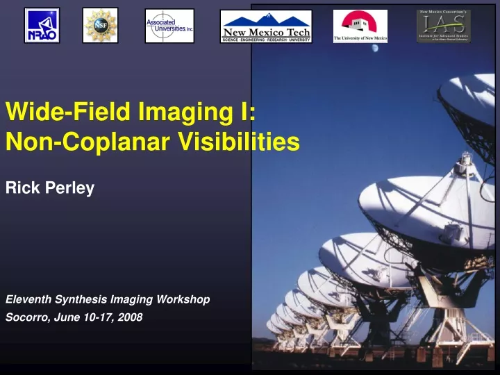
Wide-Field Imaging I: Non-Coplanar Visibilities. Rick Perley. Review: Measurement Equation. From the first lecture, we have a general relation between the complex visibility V(u,v,w), and the sky intensity I ( l , m ):. This equation is valid for:

E N D
Wide-Field Imaging I:Non-Coplanar Visibilities Rick Perley
Review: Measurement Equation • From the first lecture, we have a general relation between the complex visibility V(u,v,w), and the sky intensity I(l,m): • This equation is valid for: • spatially incoherent radiation from the far field, • phase-tracking interferometer • narrow bandwidth: • short averaging time: Eleventh Synthesis Imaging Workshop, June 10-17, 2008
Review: Coordinate Frame w The unit direction vectors is defined by its projections on the (u,v,w) axes. These components are called the Direction Cosines, (l,m,n) s n q b a v m l b The baseline vector b is specified by its coordinates (u,v,w) (measured in wavelengths). u The (u,v,w) axes are oriented so that: w points to the source center u points to the East v points to the North Eleventh Synthesis Imaging Workshop, June 10-17, 2008
When approximations fail us … • Under certain conditions, this integral relation can be reduced to a 2-dimensional Fourier transform. • This occurs when one of two conditions is met: • All the measures of the visibility are taken on a plane, or • The field of view is ‘sufficiently small’, given by: • We are in trouble when the ‘distortion-free’ solid angle is smaller than the antenna primary beam solid angle. • Define a ratio of these solid angles: Worst Case! When N2D > 1, 2-dimensional imaging is in trouble. Eleventh Synthesis Imaging Workshop, June 10-17, 2008
q2D and qPB for the VLA … • The table below shows the approximate situation for the VLA, when it is used to image its entire primary beam. • Blue numbers show the primary beam FWHM • Green numbers show situations where the 2-D approximation is safe. • Red numbers show where the approximation fails totally. Table showing the VLA’s distortion free imaging range (green), marginal zone (yellow), and danger zone (red) Eleventh Synthesis Imaging Workshop, June 10-17, 2008
Origin of the Problem is Geometry! • Consider two interferometers, with the same separation in ‘u’: One level, the other ‘on a hill’. q q q q w u u X X • What is the phase of the visibility from angle q, relative to the vertical? • For the level interferometer, • For the ‘tilted’ interferometer, • These are not the same (except when q = 0) – there is an additional phase: df = w(n-1) which is dependent both upon w and q. • The correct (2-d) phase is that of the level interferometer. Eleventh Synthesis Imaging Workshop, June 10-17, 2008
So – What To Do? • If your source, or your field of view, is larger than the ‘distortion-free’ imaging diameter, then the 2-d approximation employed in routine imaging is not valid, and you will get a distorted image. • In this case, we must return to the general integral relation between the image intensity and the measured visibilities. • This general relationship is not a Fourier transform. It thus doesn’t have an immediate inversion to the (2-d) brightness. • But, we can consider the 3-D Fourier transform of V(u,v,w), giving a 3-D ‘image volume’ F(l,m,n), and try relate this to the desired intensity, I(l,m). • The mathematical details are straightforward, but tedious, and are given in detail on pp 384-385 in the White Book. Eleventh Synthesis Imaging Workshop, June 10-17, 2008
The 3-D Image Volume F(l,m,n) • So we evaluate the following: where • and try relate the function F(l,m,n) to I (l,m). • The modified visibility V0(u,v,w) is the observed visibility with no phase compensation for the delay distance, w. • It is the visibility, referenced to the vertical direction. Eleventh Synthesis Imaging Workshop, June 10-17, 2008
Interpretation • This states that the image volume is everywhere empty (F(l,m,n)=0), except on a spherical surface of unit radius where • The correct sky image, I(l,m)/n, is the value of F(l,m,n) on this unit surface • Note: The image volume is not a physical space. It is a mathematical construct. • F(l,m,n) is related to the desired intensity, I(l,m),by: Eleventh Synthesis Imaging Workshop, June 10-17, 2008
Coordinates • Where on the unit sphere are sources found? • where d0 = the reference declination, and • Da = the offset from the reference right ascension. • However, where the sources appear on a 2-d plane is a • different matter. Eleventh Synthesis Imaging Workshop, June 10-17, 2008
Benefits of a 3-D Fourier Relation • The identification of a 3-D Fourier relation means that all the relationships and theorems mentioned for 2-d imaging in earlier lectures carry over directly. • These include: • Effects of finite sampling of V(u,v,w). • Effects of maximum and minimum baselines. • The ‘dirty beam’ (now a ‘beam ball’), sidelobes, etc. • Deconvolution, ‘clean beams’, self-calibration. • All these are, in principle, carried over unchanged, with the addition of the third dimension. • But the real world makes this straightforward approach unattractive (but not impossible). Eleventh Synthesis Imaging Workshop, June 10-17, 2008
Illustrative Example – a slice through the m = 0 plane Upper Left: True Image. Upper right: Dirty Image. Lower Left: After deconvolution. Lower right: After projection To phase center 4 sources Dirty ‘beam ball’ and sidelobes 1 2-d ‘flat’ map Eleventh Synthesis Imaging Workshop, June 10-17, 2008
Beam Balls and Beam Rays • In traditional 2-d imaging, the incomplete coverage of the (u,v) plane leads to rather poor “dirty beams’, with high sidelobes, and other undesirable characteristics. • In 3-d imaging, the same number of visibilities are now distributed through a 3-d cube. • The 3-d ‘beam ball’ is a very, very ‘dirty’ beam. • The only thing that saves us is that the sky emission is constrained to lie on the unit sphere. • Now consider a short observation from a coplanar array (like the VLA). • As the visibilities lie on a plane, the instantaneous dirty beam becomes a ‘beam ray’, along an angle defined by the orientation of the plane. Eleventh Synthesis Imaging Workshop, June 10-17, 2008
Snapshots in 3D Imaging • A deeper understanding will come from considering ‘snapshot’ observations with a coplanar array, like the VLA. • A snapshot VLA observation, seen in ‘3D’, creates ‘beam rays’ (orange lines) , which uniquely project the sources (red bars) to the tangent image plane (blue). • The apparent locations of the sources on the 2-d tangent map plane move in time, except for the tangent position (phase center). Eleventh Synthesis Imaging Workshop, June 10-17, 2008
Apparent Source Movement • As seen from the sky, the plane containing the VLA changes its tilt through the day. • This causes the ‘beam rays’ associated with the snapshot images to rotate. • The apparent source position in a 2-D image thus moves, following a conic section. The locus of the path (l’,m’) is: where Z = the zenith distance, YP= parallactic angle, and (l,m) are the correct coordinates of the source. Eleventh Synthesis Imaging Workshop, June 10-17, 2008
Wandering Sources • The apparent source motion is a function of zenith distance and parallactic angle, given by: where H = hour angle d = declination f = array latitude Eleventh Synthesis Imaging Workshop, June 10-17, 2008
Examples of the source loci for the VLA • On the 2-d (tangent) image plane, source positions follow conic sections. • The plots show the loci for declinations 90, 70, 50, 30, 10, -10, -30, and -40. • Each dot represents the location at integer HA. • The path is a circle at declination 90. • The only observation with no error is at HA=0, d=34. • The offset position scales quadraticly with source offset from the phase center. Eleventh Synthesis Imaging Workshop, June 10-17, 2008
Schematic Example m • Imagine a 24-hour observation of the north pole. The `simple’ 2-d output map will look something like this. • The red circles represent the apparent source structures. • Each doubling of distance from the phase center quadruples the extent of the distorted image. d = 90 . l Eleventh Synthesis Imaging Workshop, June 10-17, 2008
How bad is it? • The offset is (1 - cos q) tan Z ~ (q2 tan Z)/2 radians • For a source at the antenna beam first null, q ~ l/D • So the offset, e, measured in synthesized beamwidths, (l/B) at the first zero of the antenna beam can be written as • For the VLA’s A-configuration, this offset error, at the antenna beam half-maximum, can be written: e ~ lcm (tan Z)/20 (inbeamwidths) • This is very significant at meter wavelengths, and at high zenith angles (low elevations). B = maximum baseline D = antenna diameter Z = zenith distance l = wavelength Eleventh Synthesis Imaging Workshop, June 10-17, 2008
So, What Can We Do? • There are a number of ways to deal with this problem. • Compute the entire 3-d image volume via FFT. • The most straightforward approach, but hugely wasteful in computing resources! • The minimum number of ‘vertical planes’ needed is: N2D ~ Bq2/l ~ lB/D2 • The number of volume pixels to be calculated is: Npix ~ 4B3q4/l3 ~ 4lB3/D4 • But the number of pixels actually needed is: 4B2/D2 • So the fraction of the pixels in the final output map actually used is: D2/lB. (~ 2% at l = 1 meter in A-configuration!) • But – at higher frequencies, (l < 6cm?), this approach might be feasible. Eleventh Synthesis Imaging Workshop, June 10-17, 2008
Deep Cubes! • To give an idea of the scale of processing, the table below shows the number of ‘vertical’ planes needed to encompass the VLA’s primary beam. • For the A-configuration, each plane is at least 2048 x 2048. • For the New Mexico Array, it’s at least 16384 x 16384! • And one cube would be needed for each spectral channel, for each polarization! Eleventh Synthesis Imaging Workshop, June 10-17, 2008
2. Polyhedron Imaging • In this approach, we approximate the unit sphere with small flat planes (‘facets’), each of which stays close to the sphere’s surface. Tangent plane facet For each facet, the entire dataset must be phase-shifted for the facet center, and the (u,v,w) coordinates recomputed for the new orientation. Eleventh Synthesis Imaging Workshop, June 10-17, 2008
Polyhedron Approach, (cont.) • How many facets are needed? • If we want to minimize distortions, the plane mustn’t depart from the unit sphere by more than the synthesized beam, l/B. Simple analysis (see the book) shows the number of facets will be: Nf ~ 2lB/D2 or twice the number of planes needed for 3-D imaging. • But the size of each image is much smaller, so the total number of cells computed is much smaller. • The extra effort in phase shifting and (u,v,w) rotation is more than made up by the reduction in the number of cells computed. • This approach is the current standard in AIPS. Eleventh Synthesis Imaging Workshop, June 10-17, 2008
Polyhedron Imaging • Procedure is then: • Determine number of facets, and the size of each. • Generate each facet image, rotating the (u,v,w) and phase-shifting the phase center for each. • Jointly deconvolve all facets. The Clark/Cotton/Schwab major/minor cycle system is well suited for this. • Project the finished images onto a 2-d surface. • Added benefit of this approach: • As each facet is independently generated, one can imagine a separate antenna-based calibration for each. • Useful if calibration is a function of direction as well as time. • This is needed for meter-wavelength imaging at high resolution. Eleventh Synthesis Imaging Workshop, June 10-17, 2008
W-Projection • Although the polyhedron approach works well, it is expensive, as all the data have to be phase shifted, rotated, and gridded for each facet, and there are annoying boundary issues – where the facets overlap. • Is it possible to reduce the observed 3-d distribution to 2-d, through an appropriate projection algorithm? • Fundamentally, the answer appears to be NO, unless you know, in advance, the brightness distribution over the sky. • But, it appears an accurate approximation can be done, through an algorithm originated by Tim Cornwell. • This algorithm permits a single 2-d image and deconvolution, and eliminates the annoying edge effects which accompany the faceting approach. Eleventh Synthesis Imaging Workshop, June 10-17, 2008
W-Projection Basics • Consider three visibilities, measured at A, B, and C, for a source. • At A = (u0,0), for a given direction, • At B = (u0,w0), • At C = (u’ = u0-w0tanq, 0), • The visibility at B due to a source at a given direction l = sin q can be converted to the correct value at A or C simply by adjusting the phase by df = 2px, where x = w0/cosq is the propagation distance. • Visibilities propagate the same way as an EM wave! B u0,w0 w q C A u’ u0 u Eleventh Synthesis Imaging Workshop, June 10-17, 2008
W-Projection • However – to correctly project each visibility onto the plane, you need to know, in advance, the sky brightness distribution, since the measured visibility is a complex sum of visibilities from all sources: • Each component of this net vector must be independently projected onto its appropriate new position, with a phase adjustment given by the distance to the plane. • In fact, standard 2-d imaging utilizes this projection – but all visibilities are projected by the vertical distance, w. • If we don’t know the brightness in advance, we can still project the visibilities over all the cells within the field of view of interest, using the projection phase (Fresnel diffraction phase). • The maximum field of view is that limited by the antenna primary beam, q ~ l/D Eleventh Synthesis Imaging Workshop, June 10-17, 2008
W-Projection • Each visibility, at location (u,v,w) is mapped to the w=0 plane, with a phase shift proportional to the distance from the point to the plane. • Each visibility is mapped to ALL the points lying within a cone whose full angle is the same as the field of view of the desired map – ~2l/D for a full-field image. • Clearly, processing is minimized by minimizing w: Don’t observe at large zenith angles!!! w u0,w0 ~2l/D u1,w1 ~2lw0/D u0 u Eleventh Synthesis Imaging Workshop, June 10-17, 2008
Where can W-Projection be found? • The W-Projection algorithm is not (yet?) available in AIPS, but is available in CASA. • The CASA version is a trial one – it needs more testing on real data. • The authors (Cornwell, Kumar, Bhatnagar) have shown that ‘W-Projection’ is often very much faster than the facet algorithm – by over an order of magnitude in most cases. • W-Projection can also incorporate spatially-variant antenna-based phase errors – include these in the phase projection for each measured visibility. • Trials done so far give very impressive results. Eleventh Synthesis Imaging Workshop, June 10-17, 2008
An Example – without ‘3-D’ Procesesing Eleventh Synthesis Imaging Workshop, June 10-17, 2008
Example – with 3D processing Eleventh Synthesis Imaging Workshop, June 10-17, 2008
Conclusion (of sorts) • Arrays which measure visibilities within a 3-dimensional (u,v,w) volume, such as the VLA, cannot use a 2-d FFT for wide-field and/or low-frequency imaging. • The distortions in 2-d imaging are large, growing quadratically with distance, and linearly with wavelength. • In general, a 3-d imaging methodology is necessary. • Recent research shows a Fresnel-diffraction projection method is the most efficient, although the older polyhedron method is better known. • Undoubtedly, better ways can yet be found. Eleventh Synthesis Imaging Workshop, June 10-17, 2008