Download
1 / 35
360 likes | 564 Vues
Use of High-Resolution WRF Simulations to Forecast Lightning Threat. E. W. McCaul, Jr. 1 , K. La Casse 2 , S. J. Goodman 3 , and D. J. Cecil 2 1: USRA Huntsville 2: University of Alabama in Huntsville 3: NOAA/NESDIS/ORA. R3 Science Meeting Sept. 29, 2008. Photo, David Blankenship

E N D
Use of High-Resolution WRF Simulations to Forecast Lightning Threat E. W. McCaul, Jr.1, K. La Casse2, S. J. Goodman3, and D. J. Cecil2 1: USRA Huntsville 2: University of Alabama in Huntsville 3: NOAA/NESDIS/ORA R3 Science Meeting Sept. 29, 2008 Photo, David Blankenship Guntersville, Alabama
Premises and Objectives Given: Precipitating ice aloft is correlated with LTG rates Mesoscale CRMs are being used to forecast convection CRMs can represent many ice hydrometeors (crudely) Goals: Create WRF forecasts of LTG threat, based on ice flux near -15 C, vert. integrated ice, and on dBZ profile WRF: Weather Research and Forecast Model CRM: Cloud Resolving Model Additional Forecast Interests CI - convective initiation Ti - First lightning (35 dBZ at -15C, glaciation) Tp - Peak flash rate Tf - Final lightning
0 oC Flash Rate Coupled to Mass in the Mixed Phase Region Cecil et al., Mon. Wea. Rev. 2005 (from TRMM Observations)
SPC Experimental Product - Pr (CPTP) >= 1 x Pr (PCPN) >= .01” Uncalibrated probability of lightning F15 SREF 3-hr COMBINED PROBABILITY OF LIGHTNING
WRF Lightning Threat Forecasts:Methodology Use high-resolution (2-km) WRF simulations to prognose convection for a series of selected case studies Develop diagnostics from model output fields to serve as proxies for LTG: graupel fluxes; vertically integrated ice Calibrate WRF LTG proxies using peak total LTG rates from HSV LMA 4. Truncate low threat values to make threat areal coverage match LMA flash extent density obs Blend proxies to achieve optimal performance for LTG peaks and areal coverages
LTG flash rate, plotted as flash origin density, is desired parameter However, flash origin density is an extremely sparse field, and does not realistically depict spatial extent of LTG threat coverage LTG flash extent density, which accumulates counts of flashes in grid columns, with only 1 count per flash per grid column affected, gives a much more accurate spatial picture of LTG threat coverage In our graphical comparisons, we compute WRF-based LTG threat field based on calibration against actual flash origin densities; this guarantees that our peak flash rate prognoses match the observed peaks BUT… when assessing areal coverage, we compare WRF products against observed flash extent density Could calibrate WRF output against observed flash extent density, but this is too counterintuitive and complex WRF LTG Threat Forecasts: Special Issues
Compute field of graupel mixing ratio times w at -15C Plot overall peak values against observed overall peak LTG flash rates on the same grid, for a variety of cases; empirically estimate the nature of the relationship between observed LTG and its proxy; estimate any coefficients needed to convert gridded proxy to gridded LTG rate Here, we find good fit from F1 = 0.042 w qg (see next page) After applying conversion function to WRF proxy field, obtain field of LTG flash rates F1 in units of fl/(5 min)/grid column Adjust areal coverage of result to match LTG flash extent density by truncating lowest values of field of LTG threat LTG Threat 1 derived from WRF graupel flux at -15C
Prototypical Calibration Curves Threat 1 (Graupel flux)
Compute field of WRF vertically integrated ice (VII) Plot overall peak values against observed peak LTG flash rates on the same grid, for a variety of cases; empirically estimate the nature of the relationship between observed LTG, forecast proxy; estimate any coefficients needed to convert gridded proxy to gridded LTG rate Here, we find good fit from F2 = 0.20 VII (see next page) After applying conversion function to WRF proxy field, obtain field of LTG flash rates F2 in units of fl/(5 min)/grid column Adjust areal coverage of result to match LTG flash extent density by truncating lowest values of field of LTG threat LTG Threat 2 derived from WRF vertically integrated ice
Prototypical Calibration Curves Threat 2 (VII)
Methods based on LTG physics, and should be robustly useful Methods supported by solid observational evidence Can be used to obtain quantitative estimates of flash rate fields Methods are fast and simple; based on fundamental model output fields; no need for complex electrification modules Methods provide results calibrated for accurate flash rate peaks Methods include thresholds, which will allow truncation of proxy histograms so as to allow matching of areal coverages of predicted and observed LTG activity LTG Threat Methodology: Advantages
Methods are only as good as the numerical model output; model used here (WRF) has shortcomings in several areas Inherent ambiguity in interpretation of threats (extent density, etc.) Small number of cases means uncertainty in calibrations; choices of coefficient values may be off slightly, but such errors are small compared to gross model errors in storm placement Calibration requires successful simulation of both high- and low-LTG cases; the latter can be hard to find; in most cases, there are at least a few moderate or strong-LTG storms present in the domain Calibrations must be redone whenever model is changed or upgraded, or new grid is imposed LTG Threat Methodology: Disadvantages
WRF Lightning Threat Forecasts:10 December 2004Cold-season Hailstorms, Little LTG
2-km horizontal grid mesh 51 vertical sigma levels Dynamics and physics: Eulerian mass core Dudhia SW radiation RRTM LW radiation YSU PBL scheme Noah LSM WSM 6-class microphysics scheme (graupel; no hail) 8h forecast initialized at 12 UTC 10 December 2004 with AWIP212 NCEP EDAS analysis; Also used METAR, ACARS, and WSR-88D radial vel at 12 UTC; Eta 3-h forecasts used for LBC’s WRF Configuration (typical)10 December 2004 Case Study
WRF Sounding, 2004121019Z Lat=34.8 Lon=-85.9 CAPE~400
Ground truth: LTG flash extent density, dBZ10 December 2004, 19Z
WRF Lightning Threat Forecasts:30 March 2002Squall Line plus Isolated Supercell
WRF Sounding, 2002033003Z Lat=34.4 Lon=-88.1 CAPE~2800
Ground truth: LTG flash extent density, dBZ30 March 2002, 04Z
Implications of time series:1. WRF LTG threat 1 coverage too small: updrafts only2. WRF LTG threat 1 peak values have adequate t variability 3. WRF LTG threat 2 peak values have insufficient t variability because of integrating effect of multi-layer methods4. WRF LTG threat 2 coverage is good: anvil ice included5. WRF LTG threat mean biases are positive because our method of calibrating was designed to capture peak flash rates correctly, not mean flash rates6. Blend of WRF LTG threats 1 and 2 should offer good time variability, good areal coverage
Construction of blended threat:1. Threat 1 and 2 are both calibrated to yield correct peak flash densities2. The peaks of threats 1 and 2 tend to be coincident in our simulated storms, but threat 2 covers more area3. Thus, weighted linear combinations of the 2 threats will also yield the correct peak flash densities 4. To preserve most of time variability in threat 1, use large weight5. To ensure areal coverage of threat 2 is kept, small weight ok6. Tests using 0.95 for threat 1 weight, 0.05 for threat 2, yield satisfactory results
Conclusions 1:1. WRF forecasts of convection are useful, but of variable quality2. Timing of initiation of convection is depicted fairly well; however WRF convection is sometimes too widespread 3. Inclusion of WSR-88D velocity data is helpful 4. WRF convection usually deep enough, with sufficient reflectivity, to suggest lightning5. WRF wmax values on 2-km grids sometimes too weak, relative to observed weather and high-res simulations6. WRF microphysics still too simple; need more ice categories7. Finer model mesh may improve updraft representation, and hydrometeor amounts8. Biggest limitation is likely errors in initial mesoscale fields
Conclusions 2:1. These LTG threats provide more realistic spatial coverage of threat as compared to actual LTG, better than standard weather forecasts and areas covered by CAPE>02. Graupel flux LTG threat 1 is confined to updrafts, and thus underestimates LTG areal coverage; threat 2 includes anvil ice, does better3. Graupel-flux LTG threat 1 shows large time rms, like obs; VII threat 2 has small time rms 4. New blended threat can be devised that retains temporal variability of LTG threat 1, but offers proper areal coverage based on contribution from threat 2
Future Work:1. Expand catalog of simulation cases to obtain robust statistics; consider physics ensemble simulation approach2. Test newer versions of WRF, when available: - more hydrometeor species - double-moment microphysics3. Run on 1-km or finer grids; study PBL scheme response4. In future runs, examine fields of interval-cumulative wmax, and associated hydrometeor and reflectivity data, not just the instantaneous values; for save intervals of 15-30 min, events happening between saves may be important for LTG threat
Acknowledgments:This research was funded by the NASA Science Mission Directorate’s Earth Science Division in support of the Short-term Prediction and Research Transition (SPoRT) project at Marshall Space Flight Center, Huntsville, AL. Thanks also to Paul Krehbiel, NMT, Bill Koshak, NASA, Walt Petersen, UAH, formany helpful discussions