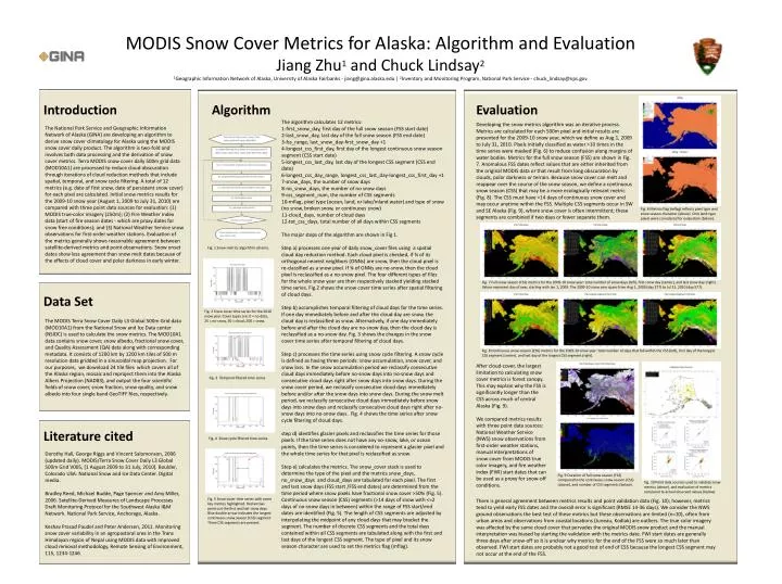
MODIS Snow Cover Metrics for Alaska: Algorithm and Evaluation Jiang Zhu 1 and Chuck Lindsay 2

1. MODIS Snow Cover Metrics for Alaska: Algorithm and Evaluation Jiang Zhu1and Chuck Lindsay2 1Geographic Information Network of Alaska, University of Alaska Fairbanks - jiang@gina.alaska.edu | 2Inventory and Monitoring Program, National Park Service - chuck_lindsay@nps.gov Introduction Algorithm Evaluation The algorithm calculates 12 metrics: 1-first_snow_day, first day of the full snow season (FSS start date) 2-last_snow_day, last day of the full snow season (FSS end date) 3-fss_range, last_snow_day-first_snow_day+1 4-longest_css_first_day, first day of the longest continuous snow season segment (CSS start date) 5-longest_css_last_day, last day of the longest CSS segment (CSS end date) 6-longest_css_day_range, longest_css_last_day-longest_css_first_day+1 7-snow_days, the number of snow days 8-no_snow_days, the number of no snow days 9-css_segment_num, the number of CSS segments 10-mflag, pixel type (ocean, land, or lake/inland water) and type of snow (no snow, broken snow, or continuous snow) 11-cloud_days, number of cloud days 12-tot_css_days, total number of all days within CSS segments The major steps of the algorithm are shown in Fig 1. Step a) processes one year of daily snow_cover files using a spatial cloud day reduction method. Each cloud pixel is checked, if ¾ of its orthogonal nearest neighbors (ONNs) are snow, then the cloud pixel is re-classified as a snow pixel. If ¾ of ONNs are no-snow, then the cloud pixel is reclassified as a no-snow pixel. The four different types of files for the whole snow year are then respectively stacked yielding stacked time series. Fig.2 shows the snow cover time series after spatial filtering of cloud days. Step b) accomplishes temporal filtering of cloud days for the time series. If one day immediately before and after the cloud day are snow, the cloud day is reclassified as snow. Alternatively, if one day immediately before and after the cloud day are no-snow day, then the cloud day is reclassified as a no-snow day. Fig. 3 shows the changes in the snow cover time series after temporal filtering of cloud days. Step c) processes the time series using snow cycle filtering. A snow cycle is defined as having three periods: snow accumulation, snow cover, and snow loss. In the snow accumulation period we reclassify consecutive cloud days immediately before no-snow days into no-snow days and consecutive cloud days right after snow days into snow days. During the snow cover period, we reclassify consecutive cloud days immediately before and/or after the snow days into snow days. During the snow melt period, we reclassify consecutive cloud days immediately before snow days into snow days and reclassify consecutive cloud days right after no-snow days into no-snow days. Fig. 4 shows the time series after snow cycle filtering of cloud days. step d) identifies glacier pixels and reclassifies the time series for those pixels. If the time series does not have any no-snow, lake, or ocean points, then the time series is considered to represent a glacier pixel and the whole time series for that pixel is reclassified as snow. Step e) calculates the metrics. The snow_cover stack is used to determine the type of the pixel and the metrics snow_days, no_snow_days and cloud_days are tabulated for each pixel. The first and last snow days (FSS start /FSS end dates) are determined from the time period where snow pixels have fractional snow cover >50% (Fig. 5). Continuous snow season (CSS) segments (>14 days of snow with <=2 days of no-snow days in between) within the range of FSS start/end dates are identified (Fig. 5). The length of CSS segments are adjusted by interpolating the midpoint of any cloud days that may bracket the segment. The number of discrete CSS segments and the total days contained within all CSS segments are tabulated along with the first and last days of the longest CSS segment. The type of pixel and its snow season character are used to set the metrics flag (mflag). Developing the snow metrics algorithm was an iterative process. Metrics are calculated for each 500m pixel and initial results are presented for the 2009-10 snow year, which we define as Aug 1, 2009 to July 31, 2010. Pixels initially classified as water >10 times in the time series were masked (Fig. 6) to reduce confusion along margins of water bodies. Metrics for the full snow season (FSS) are shown in Fig. 7. Anomalous FSS dates reflect values that are either inherited from the original MODIS data or that result from long obscuration by clouds, polar darkness or terrain. Because snow cover can melt and reappear over the course of the snow season, we define a continuous snow season (CSS) that may be a more ecologically relevant metric (Fig. 8). The CSS must have >14 days of continuous snow cover and may occur anytime within the FSS. Multiple CSS segments occur in SW and SE Alaska (Fig. 9), where snow cover is often intermittent; these segments are combined if two days or fewer separate them. The National Park Service and Geographic Information Network of Alaska (GINA) are developing an algorithm to derive snow cover climatology for Alaska using the MODIS snow cover daily product. The algorithm is two-fold and involves both data processing and the derivation of snow cover metrics. Terra MODIS snow cover daily 500m grid data (MOD10A1) are processed to reduce cloud obscuration through iterations of cloud reduction methods that include spatial, temporal, and snow cycle filtering. A total of 12 metrics (e.g. date of first snow, date of persistent snow cover) for each pixel are calculated. Initial snow metrics results for the 2009-10 snow year (August 1, 2009 to July 31, 2010) are compared with three point data sources for evaluation: (1) MODIS true-color imagery (250m); (2) Fire Weather Index data (start of fire season dates - which are proxy dates for snow free conditions); and (3) National Weather Service snow observations for first-order weather stations. Evaluation of the metrics generally shows reasonable agreement between satellite-derived metrics and point observations. Snow onset dates show less agreement than snow melt dates because of the effects of cloud cover and polar darkness in early winter. Fig. 6 Metrics flag (mflag) reflects pixel type and snow season character (above). Only land-type pixels were considered for evaluation (below). Fig. 1 Snow metrics algorithm schema. Fig. 7 Full snow season (FSS) metrics for the 2009-10 snow year: total number of snow days (left), first snow day (center), and last snow day (right). Values represent day of year, starting with Jan 1, 2009. The 2009-10 snow year spans from Aug 1, 2009 (day 277) to Jul 31, 2010 (day 577). Data Set Fig. 2 Snow cover time series for the 2010 snow year. Cover types are: 0 = no data, 25 = no-snow, 50 = cloud, 200 = snow. The MODIS Terra Snow Cover Daily L3 Global 500m Grid data (MOD10A1) from the National Snow and Ice Data center (NSIDC) is used to calculate the snow metrics. The MOD10A1 data contains snow cover, snow albedo, fractional snow cover, and Quality Assessment (QA) data along with corresponding metadata. It consists of 1200 km by 1200 km tiles of 500 m resolution data gridded in a sinusoidal map projection. For our purposes, we download 24 tile files which covers all of the Alaska region, mosaic and reproject them into the Alaska Albers Projection (NAD83), and output the four scientific fields of snow cover, snow fraction, snow quality, and snow albedo into four single band GeoTIFF files, respectively. Fig. 8 Continuous snow season (CSS) metrics for the 2009-10 snow year: total number of days that fall within the CSS (left), first day of the longest CSS segment (center), and last day of the longest CSS segment (right). After cloud-cover, the largest limitation to calculating snow cover metrics is forest canopy. This may explain why the FSS is significantly longer than the CSS across much of central Alaska (Fig. 9). We compared metrics results with three point data sources: National Weather Service (NWS) snow observations from first-order weather stations, manual interpretations of snow cover from MODIS true color imagery, and fire weather index (FWI) start dates that can be used as a proxy for snow-off conditions. Fig. 3 Temporal filtered time series. Literature cited Fig. 4 Snow cycle filtered time series. • Dorothy Hall, George Riggs and Vincent Salomonson, 2006 (updated daily). MODIS/Terra Snow Cover Daily L3 Global 500m Grid V005, [1 August 2009 to 31 July, 2010]. Boulder, Colorado USA: National Snow and Ice Data Center. Digital media. • Bradley Reed, Michael Budde, Page Spencer and Amy Miller, 2006. Satellite-Derived Measures of Landscape Processes Draft Monitoring Protocol for the Southwest Alaska I&M Network. National Park Service, Anchorage, Alaska. • KeshavPrasad Paudel and Peter Andersen, 2011. Monitoring snow cover variability in an agropastoral area in the Trans Himalayan region of Nepal using MODIS data with improved cloud removal methodology, Remote Sensing of Environment, 115, 1234-1246. Fig. 9 Duration of full snow season (FSS) compared to the continuous snow season (CSS) (above), and number of CSS segments (below). Fig. 10 Point data sources used to validate snow metrics (above), and evaluation of metrics compared to actual observed values (below). Fig. 5 Snow cover time series with some key metrics highlighted. Red arrows point out the first and last snow days. Blue double arrow indicates the longest continuous snow season (CSS) segment. Three CSS segments are present. There is general agreement between metrics results and point validation data (Fig. 10); however, metrics tend to yield early FSS dates and the overall error is significant (RMSE 14-36 days). We consider the NWS ground observations the best test of these metrics but these observations are limited (n=10), often from urban areas and observations from coastal locations (Juneau, Kodiak) are outliers. The true color imagery was affected by the same cloud cover that pervades the original MODIS snow product and the manual interpretation was biased by starting the validation with the metrics date. FWI start dates are generally three days after snow-off so it is unclear why metrics for the end of the FSS were so much later than observed. FWI start dates are probably not a good test of end of CSS because the longest CSS segment may not occur at the end of the FSS.