Download
1 / 45
710 likes | 1.6k Vues
SECTION 1 HEAT TRANSFER ANALYSIS. THERMAL ANALYSIS WITH MSC.MARC. Why a Structural Analyst may have to perform Thermal Analysis Modes of Heat Transfer Available in MSC.Marc and MSC.Patran support Conduction Convection Radiation Transient Analysis versus Steady State Analysis.

E N D
SECTION 1 HEAT TRANSFER ANALYSIS
Why a Structural Analyst may have to perform Thermal Analysis Modes of Heat Transfer Available in MSC.Marcand MSC.Patran support Conduction Convection Radiation Transient Analysis versus Steady State Analysis Linear versus Nonlinear Minimum Allowable Time Increment Thermal Analysis How to calculate it Physical Interpretation What happens if you violate the formula Sequentially Coupled Problems versus Fully Coupled Problems OVERVIEW
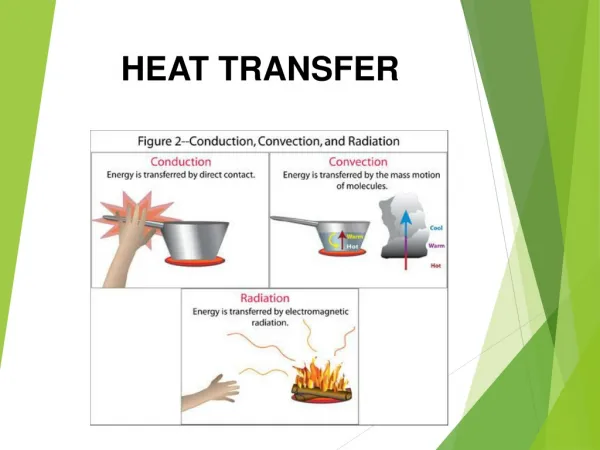
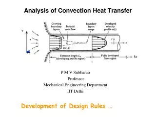
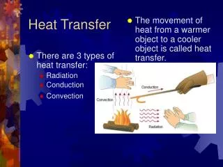
T1 q T2 T2 q q1 q T1 T1 T1 T2 T2 q2 Moving Fluid Removes Heat From Solid T1>T2 Heat Moves IN Moving Fluid T1>T2 T1>T2 T1>T2 Conduction Convection HEAT TRANSFER Motivation • When the solution for the temperature field in a solid (or fluid) is desired, and the temperature is not influenced by the other unknown fields, a heat transfer analysis is appropriate. q= -k [dT/dx] Advection Radiation Modes of Heat Transfer
HEAT TRANSFER MODES Motivation When the solution for the temperature field in a solid (or fluid) is desired,and is not influenced by the other unknown fields, heat transfer analysis is appropriate. • Conduction • Convection • Radiation • Contact Heat Transfer:
HEAT TRANSFER • Steady State Heat Transfer • Definition • Heat transfer analysis is used to determine the temperature field of a given structure. It can also be used as a starting point in a thermal expansion analysis. This is a structural analysis where the applied load is temperature.
HEAT TRANSFER • Objective • To determine the temperature field of a structure. • Secondary results of interest include heat flux. • Assumptions • The typical heat transfer problem is a conduction problem where convections and radiation are boundary conditions.
HEAT TRANSFER • Some terms to keep in mind. • Flux: the rate of energy flow across a surface. Denoted by a symbol q’’ = q flux. (單位時間單位面積通過的熱量或能量)(通量) • Energy: amount of usable power. In this case we are talking about heat as the usable power. So energy would be the flux times the area of the surface times time. (熱傳的能量指熱量) • Heat: energy in transit due to a temperature difference. This is also called heat transfer. (熱量) • Modes of Heat Transfer:Conduction, Convection, Radiation
T T1 T(x) q out q in T2 x HEAT TRANSFER • Conduction: Internal energy transfer due to thermal gradients interior to a body or across perfect contact of two bodies. K is a given property of the material. q = q” x A Analysis is converged when the heat flow is balanced qin – qout = 0 (steady State)
HEAT TRANSFER • Conduction (cont’d) where, • q is the heat-transfer rate (heat per unit time) • k is the thermal conductivity (power per distance temperature) • A is the area normal to the heat flow • T is the temperature • x is the direction of heat flow (conduction flux)
HEAT TRANSFER • Convection: Energy transfer between a solid body and a surrounding fluid (gas or liquid). TBor q hf is either a) given from the geometry of the body and the state of the fluid or b) the result of a thermal CFD analysis. hf is called the convection coefficient. Used mainly as a boundary condition so the user would input hf and TB. TS
HEAT TRANSFER • Convection where, • q” is the heat-transfer rate per unit area • hf is the convective film coefficient • TS is the surface temperature • TB is the bulk temperature • A is the area that the heat is transferred across
i j Q Electromagnetic wave HEAT TRANSFER • Radiation: Energy transfer by electromagnetic waves. σ = 5.67E-8 W / m² • = 0.1714E-8 Btu / h • ft² • Fij is solved for each element pair.This is done before the solution is run and may be either automated or a user input.
HEAT TRANSFER • Radiation where, • q is the heat flow rate from surface i to j. • σ is the Stephan-Boltzman constant • ε is the emissivity (放射率) • Ai is the area of surface i • Fij is the form factor between surfaces i & j • Ti, Tj are the absolute temperatures of the surfaces
Insulated boundaries E out E in Q Insulated boundaries HEAT TRANSFER • Equation of State: 1D Example • We will first derive the basic differential equation for the one dimensional conduction only problem. This will allow us an insight to the physical problem that is needed before that FEA formulation is understood. • Begin with the conservation of energy and apply it to a control volume. E in + E generated = E out + U (change in stored energy)
HEAT TRANSFER Ein is the energy entering the volume in units of J (joules). qx” is the conduction heat flux into the volume Ein = q”x • A • dt = qx • dt (flux | power into system) Eout = q”x+dx • A • dt = qx+dx • dt (flux | power out of system) Egenerated = Q • A • dx • dt (power per unit volume) Q is the internal heat source 1 J = 1 N • M A is the cross sectional area of the control volume
dx qx+dx Q qx area A HEAT TRANSFER • Put all the parts together: • Use Fourier’s Law: EQ 1
HEAT TRANSFER • And apply Taylor’s Expansion Theorem • This results in • Stored energy term U = (specific heat) x (mass) x (change in temperature)
HEAT TRANSFER • Substituting the preceding into the energy balance equation (eq 1), we have • Simplifying and dividing by Adxdt we are left with: 0 for steady state
HEAT TRANSFER • For steady state, any differential with respect to time is zero. Also assume that the conductivity of the material is constant. • The following boundary conditions are possible • 1) T = Tb, Tb would be a known temperature DOF constraint • 2) = constant. This is a prescribed heat flux. • 3)on an insulated boundary. This is the “natural” boundary condition.It exists if nothing is applied. steady state conduction Add/subtract energy
qh area A qx+dx Q qx dx HEAT TRANSFER • Now convection can be added. • The convection replaces the insulated boundary from before. qh acts on an area therefore let P be the perimeter around area A.
HEAT TRANSFER • Add this term to EQ 1 and simplify as before: EQ2
HEAT TRANSFER • Again, assume no time dependence and a constant conduction coefficient: • Now one more boundary condition can be added to the previous three: • 4) the heat flow at the solid/surface interface is balanced.
HEAT TRANSFER • Transient Heat Transfer • Definition • Heat transfer analysis where the temperature of the structure is now a function of time. • Don’t forget to add density, , and specific heat, , to the material definition.
HEAT TRANSFER • Special Topics • Non-Linear Heat Transfer • Examine the heat equation (no radiation) if the material properties are functions of temperature, the analysis is non-linear (in temp).
HEAT TRANSFER • Special Topics • Non-Linear Heat Transfer - Radiation • Add the radiation flux term to EQ 2 (acts over the same surface area as convection) radiation is naturally non-linear as it depends on the fourth power of temperature. Emissivity may also be a function of temp.
q”x Ta q”gap B q”contact Tb HEAT TRANSFER • Special Topics • Thermal Contact Resistance • Where two structures meet, the temperature drop across the interface may be appreciable. The temperature difference results from the fact that on a microscopic (or not so micro) scale, the surfaces are not in perfect contact i.e. gaps exist.
HEAT TRANSFER • Special Topics • Thermal Contact Resistance • The resistance due to thermal contact is defined as: (R=1/hA) most values of R” are derived experimentally which is more reliable than the current theories for predicting R”.
HEAT TRANSFER • Summary • 1D Steady State Definitions and Examples • Conduction • Convection • Radiation • Derivation of state equation • Transient Heat Transfer • Special Topics • Non-linear Heat Transfer • Thermal Contact Resistance • Units
HEAT TRANSFER EXAMPLE • Example:Steady State Analysis of Radiator(Workshop 4) Convection given about connector Temperature given at bottom left and right end surfaces Computed Temperatures
HEAT TRANSFER MATHEMATICS • Energy flow density is given by a diffusion and convection part: • Thermal equilibrium between heat sources, energy flow density and temperature rate is expressed by the Energy Conservation Law, which may be written: where is L is the conductivity matrix. Assume that the continuum is incompressible and that there is no spatial variation of r and Cp; then the conservation law becomes:
HEAT TRANSFER LOADS & BOUNDARY CONDITIONS (CONT.) 6) Contact conduction: contact h : Transfer coeff. = Temp.Body 2 = Temp.Body 1
Only in transient analysis: MSC.Marc uses a backward difference scheme to approximate the time derivative as: . T = where resulting in the finite difference scheme: C: heat capacity matrix K: conductivity and convection matrix F: contribution from convective boundary condition : vector of nodal fluxes HEAT TRANSFER INITIAL CONDITIONS
THERMAL RADIATION • New Radiation LBC • Radiation Viewfactor calculation • Uses Monte Carlo Simulation • 2D • Axisymmetric • 3D • New Convective Velocity LBC • Thermal or Coupled analysis
RADIATION OVERVIEW Basic equation: q = s F A (Ti4 – Tj4) • T is in absolute units • Kelvin or Rankine • s is the Stefan Boltzmann Constant • 5.6696E-8 Watt/(m2-K4) • 1.7140E-9 Btu/(hr-ft2-R4) • F (script-F) is the gray body configuration factor • F is a function of • Fij, the geometric view-factor from surface-i to surface-j • ei, the emissivity of surface-i • ej, the emissivity of surface-j
1-ei 1-ej 1 eiAi ejAj AiFij RADIOSITY CONCEPT • Radiosity node added for each surface node (e < 1.0) • FA is separated into two terms • A “space” resistancewhich is a function of only Fij • Each “surface” resistance a function of either ei and ejonly • This technique facilitates • Change in surface properties (e) without new view factor run • Independently variable emissivity values • e = 1.0 will eliminate radiosity nodes • Facilitates debugging of surface-to-surface connections Eb1 J2 Eb2 J1
HEAT TRANSFER IN MSC.PATRAN MARC PREFERENCE • All three modes of heat transfer may be present in an MSC.Marc analysis. There are two basic types of analyses: • Transient analysis: to obtain the history of the response over time with heat capacity and latent heat effects taken into account • Steady state analysis: when only the long term solution under a given set of loads and boundary conditions is sought (No heat accumulation).
Temperature Time THERMAL NONLINEAR ANALYSES • Either type of thermal analysis can be nonlinear. • Sources of nonlinearity include: • Temperature dependence of material properties. • Nonlinear surface conditions: e.g. radiation, temperature dependent film (surface convection) coefficients. • Loads which vary nonlinearly with temperature. These loads are described using Fields in MSC.Patran. • Latent heat (phase change) effects
HEAT TRANSFER SHELL ELEMENT • Prior to version 2001, shell elements could have a linear or a quadratic temperature distribution in thickness direction; per node, the number of degrees of freedom is: 2: top and bottom surface temperature (linear) 3: top, bottom and mid surface temperature (quadratic) • Especially for certain composite structures, a linear or quadratic distribution might be insufficient to accurately describe the actual temperature profile
HEAT TRANSFER SHELL ELEMENT (CONT.) • New in version 2001: take a linear or quadratic temperature profile per layer ; per node, the number of degrees of freedom is: • M+1 (M = # of composite layers; linear distribution): 1 = top surface temperature 2 = temperature at layer 1-2 interface 3 = temperature at layer 2-3 interface … M+1 = bottom surface temperature • 2*M+1 (M = # of composite layers; quadratic distribution): 1 = top surface temperature 2 = temperature at layer 1-2 interface 3 = mid surface temperature of layer 1 4 = temperature at layer 2-3 interface … 2*M+1 = mid surface temperature layer M • The new temperature distribution can also be user for non-composite elements
FULLY COUPLED PROBLEMS • Thermal field affects the mechanical field as above • Thermal loads induce deformation. • Mechanical field affects thermal field • Mechanically generate heat-due to plastic work or friction • Deformation changes modes of conduction, radiation, etc. • Fully coupled problems are supported in MSC.Marc 2001 but not by MSC.Patran 2001 • Fully coupled problems are supported in MSC.Patran 2002