Download
1 / 67
680 likes | 802 Vues
Quality Management “ It costs a lot to produce a bad product. ” Norman Augustine. Cost of quality. Prevention costs Appraisal costs Internal failure costs External failure costs Opportunity costs. What is quality management all about?.

E N D
Quality Management “It costs a lot to produce a bad product.”Norman Augustine
Cost of quality • Prevention costs • Appraisal costs • Internal failure costs • External failure costs • Opportunity costs
What is quality management all about? Try to manage all aspects of the organization in order to excel in all dimensions that are important to “customers” Two aspects of quality: features: more features that meet customer needs = higher quality freedom from trouble: fewer defects = higher quality
The Quality Gurus – Edward Deming • Quality is “uniformity and dependability” • Focus on SPC and statistical tools • “14 Points” for management • PDCA method 1900-1993 1986
The Quality Gurus – Joseph Juran • Quality is “fitness for use” • Pareto Principle • Cost of Quality • General management approach as well as statistics 1904 - 2008 1951
Defining Quality The totality of features and characteristics of a product or service that bears on its ability to satisfy stated or implied needs American Society for Quality
MNBQA Leadership: How upper management leads the organization, and how the organization leads within the community. Strategic planning: How the organization establishes and plans to implement strategic directions. Customer and market focus: How the organization builds and maintains strong, lasting relationships with customers. Measurement, analysis, and knowledge management:How the organization uses data to support key processes and manage performance. Human resource focus: How the organization empowers and involves its workforce. Process management:How the organization designs, manages and improves key processes. Business/organizational performance results: How the organization performs in terms of customer satisfaction, finances, human resources, supplier and partner performance, operations, governance and social responsibility, and how the organization compares to its competitors.
Technical Tools (Process Analysis, SPC, QFD) Customer Cultural Alignment What does Total Quality Management encompass? • TQM is a management philosophy: • continuous improvement • leadership development • partnership development
Design quality Dimensions of quality Conformance quality Developing quality specifications Design Input Process Output
Quality Improvement Continuous Improvement Quality Traditional Time
Plan Do Act Check Continuous improvement philosophy • Kaizen: Japanese term for continuous improvement. A step-by-step improvement of business processes. • PDCA: Plan-do-check-act as defined by Deming. • Benchmarking : what do top performers do?
Tools used for continuous improvement 1. Process flowchart
Performance Time Tools used for continuous improvement 2. Run Chart
Tools used for continuous improvement 3. Control Charts Performance Metric Time
Machine Man Environment Method Material Tools used for continuous improvement 4. Cause and effect diagram (fishbone)
Tools used for continuous improvement 5. Check sheet
Frequency Tools used for continuous improvement 6. Histogram
Tools used for continuous improvement 7. Pareto Analysis 100% 60 75% 50 40 Frequency 50% Percentage 30 20 25% 10 0% A B C D E F
A philosophy and set of methods companies use to eliminate defects in their products and processes Seeks to reduce variation in the processes that lead to product defects The name “six sigma” refers to the variation that exists within plus or minus six standard deviations of the process outputs Six Sigma Quality
Absent receiving party Working system of operators Absent Too many phone calls Lunchtime Out of office Makes customer wait Not at desk Absent Not giving receiving party’s coordinates Does not understand customer Lengthy talk Does not know organization well Complaining Takes too much time to explain Leaving a message Customer Operator Fishbone diagram analysis
Reasons why customers have to wait (12-day analysis with check sheet)
Frequency Percentage 87.1% 300 250 71.2% 200 49% 150 100 0% A B C D E F Pareto Analysis: reasons why customers have to wait
In general, how can we monitor quality…? By observing variation in output measures! • Assignable variation: we can assess the cause • Common variation: variation that may not be possible to correct (random variation, random noise)
Statistical Process Control (SPC) • Control Charts for Variables • The Central Limit Theorem • Setting Mean Chart Limits (x-Charts) • Setting Range Chart Limits (R-Charts) • Using Mean and Range Charts • Control Charts for Attributes • Managerial Issues and Control Charts SPC – suppl ch. 6
Variability is inherent in every process Natural or common causes Special or assignable causes Provides a statistical signal when assignable causes are present Detect and eliminate assignable causes of variation Statistical Process Control (SPC)
Each of these represents one sample of five boxes of cereal # # # # # Frequency # # # # # # # # # # # # # # # # # # # # # Weight Samples To measure the process, we take samples and analyze the sample statistics following these steps (a) Samples of the product, say five boxes of cereal taken off the filling machine line, vary from each other in weight Figure S6.1
The solid line represents the distribution Frequency Weight Samples To measure the process, we take samples and analyze the sample statistics following these steps (b) After enough samples are taken from a stable process, they form a pattern called a distribution Figure S6.1
Central tendency Variation Shape Frequency Weight Weight Weight Samples To measure the process, we take samples and analyze the sample statistics following these steps (c) There are many types of distributions, including the normal (bell-shaped) distribution, but distributions do differ in terms of central tendency (mean), standard deviation or variance, and shape Figure S6.1
Prediction Frequency Time Weight Samples To measure the process, we take samples and analyze the sample statistics following these steps (d) If only natural causes of variation are present, the output of a process forms a distribution that is stable over time and is predictable Figure S6.1
? ? ? ? ? ? ? ? ? ? ? ? ? ? ? ? ? ? ? Prediction Frequency Time Weight Samples To measure the process, we take samples and analyze the sample statistics following these steps (e) If assignable causes are present, the process output is not stable over time and is not predicable Figure S6.1
Control Charts Constructed from historical data, the purpose of control charts is to help distinguish between natural variations and variations due to assignable causes
Types of Data Variables Attributes • Characteristics that can take any real value • May be in whole or in fractional numbers • Continuous random variables • Defect-related characteristics • Classify products as either good or bad or count defects • Categorical or discrete random variables
(a) In statistical control and capable of producing within control limits Frequency Upper control limit Lower control limit (b) In statistical control but not capable of producing within control limits (c) Out of control Size (weight, length, speed, etc.) Process Control Figure S6.2
Three population distributions Mean of sample means = x Beta Standard deviation of the sample means Normal = sx = Uniform s n | | | | | | | -3sx -2sx -1sx x +1sx +2sx +3sx 95.45% fall within ± 2sx 99.73% of all x fall within ± 3sx Population and Sampling Distributions Distribution of sample means Figure S6.3
Sampling distribution of means Process distribution of means x = m (mean) Sampling Distribution Figure S6.4
For variables that have continuous dimensions • Weight, speed, length, strength, etc. • x-charts are to control the central tendency of the process • R-charts are to control the dispersion of the process • These two charts must be used together Control Charts for Variables
For x-Charts when we know s Upper control limit (UCL) = x + zsx Lower control limit (LCL) = x - zsx where x = mean of the sample means or a target value set for the process z = number of normal standard deviations sx = standard deviation of the sample means = s/ n s = population standard deviation n = sample size Setting Chart Limits
Hour 1 Sample Weight of Number Oat Flakes 1 17 2 13 3 16 4 18 5 17 6 16 7 15 8 17 9 16 Mean 16.1 s = 1 Hour Mean Hour Mean 1 16.1 7 15.2 2 16.8 8 16.4 3 15.5 9 16.3 4 16.5 10 14.8 5 16.5 11 14.2 6 16.4 12 17.3 n = 9 UCLx = x + zsx= 16 + 3(1/3) = 17 ozs LCLx = x - zsx = 16 - 3(1/3) = 15 ozs Setting Control Limits For 99.73% control limits, z = 3
Variation due to assignable causes Out of control 17 = UCL Variation due to natural causes 16 = Mean 15 = LCL Variation due to assignable causes | | | | | | | | | | | | 1 2 3 4 5 6 7 8 9 10 11 12 Out of control Sample number Setting Control Limits Control Chart for sample of 9 boxes
For x-Charts when we don’t know s Upper control limit (UCL) = x + A2R Lower control limit (LCL) = x - A2R where R = average range of the samples A2 = control chart factor found in Table S6.1 x = mean of the sample means Setting Chart Limits
Sample Size Mean Factor Upper Range Lower Range n A2D4D3 2 1.880 3.268 0 3 1.023 2.574 0 4 .729 2.282 0 5 .577 2.115 0 6 .483 2.004 0 7 .419 1.924 0.076 8 .373 1.864 0.136 9 .337 1.816 0.184 10 .308 1.777 0.223 12 .266 1.716 0.284 Control Chart Factors Table S6.1
Process average x = 16.01 ounces Average range R = .25 Sample size n = 5 Setting Control Limits
Process average x = 16.01 ounces Average range R = .25 Sample size n = 5 UCLx = x + A2R = 16.01 + (.577)(.25) = 16.01 + .144 = 16.154 ounces From Table S6.1 Setting Control Limits
Process average x = 16.01 ounces Average range R = .25 Sample size n = 5 UCLx = x + A2R = 16.01 + (.577)(.25) = 16.01 + .144 = 16.154 ounces UCL = 16.154 Mean = 16.01 LCLx = x - A2R = 16.01 - .144 = 15.866 ounces LCL = 15.866 Setting Control Limits
R – Chart • Type of variables control chart • Shows sample ranges over time • Difference between smallest and largest values in sample • Monitors process variability • Independent from process mean
Upper control limit (UCLR) = D4R Lower control limit (LCLR) = D3R where R = average range of the samples D3 and D4 = control chart factors from Table S6.1 Setting Chart Limits For R-Charts
Average range R = 5.3 pounds Sample size n = 5 From Table S6.1 D4= 2.115, D3 = 0 UCLR = D4R = (2.115)(5.3) = 11.2 pounds UCL = 11.2 Mean = 5.3 LCLR = D3R = (0)(5.3) = 0 pounds LCL = 0 Setting Control Limits
(a) These sampling distributions result in the charts below (Sampling mean is shifting upward but range is consistent) UCL (x-chart detects shift in central tendency) x-chart LCL UCL (R-chart does not detect change in mean) R-chart LCL Mean and Range Charts Figure S6.5
(b) These sampling distributions result in the charts below (Sampling mean is constant but dispersion is increasing) UCL (x-chart does not detect the increase in dispersion) x-chart LCL UCL (R-chart detects increase in dispersion) R-chart LCL Mean and Range Charts Figure S6.5