Download
1 / 95
980 likes | 1.22k Vues
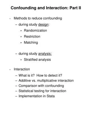
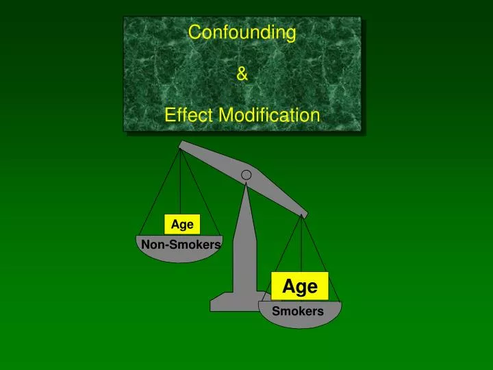
Age. Age. Confounding & Effect Modification. Non-Smokers. Smokers. 20 108 128 15.6%. Yes. Heart Disease. Yes No. Incidence. Vigorous Exercise. 30 64 94 31.9%. No. RR (95% CI)= 0.5 (0.3-0.8)

E N D
Age Age Confounding&Effect Modification Non-Smokers Smokers
20 108 128 15.6% Yes Heart Disease Yes No Incidence Vigorous Exercise 30 64 94 31.9% No RR (95% CI)= 0.5 (0.3-0.8) p = 0.004
Age Age Active Age Age Active Active Active Sedentary Sedentary Age Sedentary Age Sedentary Unequal Age Distribution Exaggerates the Benefit of Exercise Weighing the Risk of CAD Equal Ages Provide a Fairer Comparison
Confounding (Latin: “confundere” : to mix together) The true effect of the exposure on likelihood of disease is distorted because it is mixed up with another factor that is associated with the disease. Older people exercise less. age Older people have more risk of heart disease. ? physical inactivity heart disease Confounding occurs when the study groups differ with respect to other factors that influence the outcome. What is the relationship after removing the distorting effect of confounding by age?
In order for confounding to occur the extraneous factor must be associated with both the risk factor being evaluated and the outcome of interest. fluid intake ? coronary artery disease physical inactivity Even if fluid intake differs, it will not confound this relationship, since it doesn’t affect CAD.
age Older people have more risk of heart disease. ? physical inactivity heart disease However, if the age distributions of the groups being compared are the same, there will be no confounding.
Alaska Florida Confounding Confounding occurs when the study groups differ with respect to other factors that influence the outcome. This distorts the association you are trying to evaluate. Age Age The comparison of cancer death rates in Alaska & Florida was distorted by the older age distribution in Florida. This was dealt with by calculating “age-adjusted” rates which removed the effect of age differences.
Confounding Can Exaggerate Differences… Apparent difference (Crude, Unadjusted) Confounding may account for allorpart of an apparent association. True difference (Adjusted) True difference (Adjusted)
…or Confounding Can Cause Differences to Be Underestimated Apparent difference (Crude, Unadjusted) Confounding may account for all or part of an apparent association. Difference after Adjusting
Age Active Age Sedentary Confounders are other risk factors that confuse the relationship you want to study, so you want to remove their effect. The comparison of CAD was distorted by the fact that sedentary subjects may be older. Goal: determine the association between activity and heart disease after removing the distorting effect of age.
Active Sedentary Fam Hx Diabetes Fam Hx Age Diabetes Age Other Differences BetweenExercisers and Non-exercisers Active Sedentary Age 46 + 1.4 59 + 1.5 Body Fat % 15 + 4.5 22 + 5.6 Dietary fat % 29 + 5.0 42 + 7.0 Current smokers 5% 24% Hypertension 8% 17% Diabetes mellitus 2% 9% Family history of CHD 25% 5% Males 60% 40% Confounders are other risk factors or preventive factors for the outcome of interest.
Ways to Control for Confounding • In the Design: • Restriction • Matching (also need matched analysis) • Randomization (don’t need to know • what the confounders are) • In the Analysis: • Stratification • Multivariate Analysis
Restriction We could restrict our study on exercise to non-smoking, non-diabetic, white males age 20-40. • Simple and effective, but • There will be residual confounding if restriction is not narrow enough. • Limits sample size. • Can’t evaluate restricted variable. • Limits ability to generalize findings.
Matching • Simple and effective, but • Expensive, time-consuming • Limits sample size • You can’t evaluate the matched factor. • Very Useful For: • - complex multifaceted variables (e.g., environment, heredity) • - case-control with few cases, but many controls (e.g., DES)
Randomization (in a clinical trial) • Subjects are allocated to treatment groups by a random method that gives an equal chance of being in any treatment group. • With adequate numbers of subjects, it insures baseline comparability of groups. • Provides control for both known and unknown confounders.
Control of Confounding (in analysis)Stratification age ? physical inactivity coronary artery disease • Older people tend to exercise less. • Older people have a greater risk of heart disease. If differences between young and old confuse the relationship between physical activity and coronary artery disease, then look at the relationship separately in the young and the old.
Heart Disease yes no Confounding in a Cohort Study 48 800 69 625 yes Active no Crude RR = 0.57 Stratified Analysis Young subjects (<45) Older subjects Heart Disease yes no Heart Disease yes no 23 200 58 400 25 600 11 225 yes Active no Ie=0.040 Io=0.047 Ie=0.10 Io=0.13 yes Active no RR = 0.86 RR = 0.81 The stratum-specific RRs differ from crude, but are similar to each other (confounding). There’s a benefit of activity, but not as great as the crude RR suggested.
Summarizing Results of Stratified Analysis Young subjects (<45) Older subjects Heart Disease yes no Heart Disease yes no 23 200 58 400 25 600 11 225 yes Active no yes Active no RR = 0.86 RR = 0.81 Mantel-Haenszel Equations Calculate: A pooled average of the stratum-specific RRs. RRmh = 0.84 (adjusted for confounding by age) Mantel-Haenszel chi-square test: tests significance of the adjusted RR.
35-39 40-44 45-49 50-54 55-59 60-64 Multiple Strata to Control for Confounding by Age Heart Disease + - Exercise + - RR=0.5 (Crude RR) RR: 0.72 0.81 0.80 0.79 0.83 0.77 (Stratum-specific Relative Risks) Pooled estimate: RRmh= 0.79)
Family History Family History of Heart Disease Negative Males Females Males Females Multiple Strata to Control for Confounding by Two Factors (or more) Heart Disease + - Exercise + -
Effect Modification in a Cohort Study Heart Disease yes no 51 800 76 600 yes Active no Crude RR = 0.57 Stratified Analysis Men Women Heart Disease yes no Heart Disease yes no 11 339 9 341 35 315 60 290 yes Active no yes Active no RR = 0.58 (0.40 - 0.86) RR = 1.22 (0.51 - 2.91) The effect of exercise on heart disease is different in men and women. Effect modification is present if the stratum-specific estimates of association differ from each other!
Heart Disease yes no Effect Modification in a Cohort Study 51 800 76 600 yes Active no Crude RR = 0.57 Stratified Analysis Men Women Heart Disease yes no Heart Disease yes no 11 339 9 341 35 315 60 290 yes Active no yes Active no RR = 0.58 (0.40 - 0.86) RR = 1.22 (0.51 - 2.91) Possible explanations: 1) The effect of exercise on risk of heart disease is different in men and women, i.e. there is a physiologic difference. (Effect modification) 2) Inadequate sample size & imprecise estimates.
Effect Modification “Interaction” or “Synergism” When the magnitude of association (effect) is modified by another factor. Example: The association between smoking and lung cancer is modified by asbestos exposure. Without Asbestos With Asbestos Lung Cancer Lung Cancer RR = 20 RR = 64 Y N Y N Y Y Smoking Smoking N N
Is there an association between smoking and lung cancer? Lung Cancer Y N Y RR = 26 Smoking N 50-59 year olds 60-69 year olds Lung Cancer Lung Cancer RR = 20 RR = 21 Y N Y N Y Y Smoking Smoking N N
26 600 11 200 Heart Disease yes no Both Effect Modification & Confounding 54 800 69 600 yes Active no Crude RR = 0.61 Stratified Analysis Young Old Heart Disease yes no Heart Disease yes no 28 200 58 400 yes Active no yes Active no RR = 0.80 (0.50 - 1.10) RR = 0.97 (0.57 - 1.37) Stratum-specific estimates of association differ from crude estimate and also differ from each other!
Stratified Analysis: Summary • Purposes: • Identify & control for confounding • Identify effect modification • Possibilities: • 1) No confounding or effect modification • 2) Confounding only • 3) Effect modification only • 4) Both effect modification & confounding
Effect Modification Like confounding, effect modification can be evaluated by stratification. BUT Effect modification is a biological phenomenon that should be carefully described (not adjusted for). When the stratum-specific estimates differ: Report the stratum-specific estimates of association and the 95% confidence interval for each. Do NOT combine the stratum-specific estimates into a pooled estimate.
“Eyeball” the Results • If crude and stratum-specific estimates of RR are similar, • there is no confounding or effect modification • If stratum-specific estimates differ appreciably from each • other then effect modification is occurring & should be • described by reporting all stratum-specific estimates • separately. • If stratum-specific RRs differ from crude, but are similar to • one another, then confounding has occurred, and an • adjusted estimate should be calculated (Mantel-Haentzel). The 10% Rule
Dietary Fiber and Colon Cancer A case-control study was done to look for an association between low dietary fiber and risk of colon cancer. Crude analysis: OR= 3.1 95% CI: 1.2-4.2 Stratified by dietary fat content: High Fat Low Fat Cancer yes no Cancer yes no yes Low Fiber no yes Low Fiber no OR = 1.1 (0.60 - 1.95) OR = 1.2 (0.50 - 1.90)
A Cohort Study Is High BMI Associated with CHD? Given: Age is associated with both high BMI & risk of CHD. Crude CHD No CHD Totals Incidence High BMI 220 9,780 10,000 .022 Low BMI 83 9,917 10,000 .0083 Crude RR = 2.65 Young CHD No CHD Totals Incidence High BMI 20 3,980 4,000 .005 Low BMI 18 6,982 7,000 .00257 RR = 1.94 Old CHD No CHD Totals Incidence High BMI 200 5,800 6,000 .0333 Low BMI 65 2,935 3,000 .02167 RR = 1.54 • Is age a confounder in this study? • Is there effect modification?
The Problem of Multiple Confounding Factors • Stratify by: • gender • age (5 categories) • smoking status (never, former, current) males females 5 ages 5 ages 3 levels of smoking for each age & gender group 30 different sub-strata!!! (some with very small # of subjects)
Death yes no yes 70+ no 13 61 25 935 74 960 Stratified Analysis Death yes no Death yes no No Safety (Unrestrained) Various Safety yes 70+ no 5 45 12 576 8 16 13 359 yes 70+ no To evaluate confounding, you can use Mantel-Haenszel method to compute a pooled average, then see if this differs from crude RR by >10% RRmh=7.22 (7.22-6.75)/6.75 = 0.07 =7% RR = 4.90 RR = 9.54 MVC 17.6% 2.6% Crude RR = 6.75 33.1% 3.5% 10 % 2 %
The Problem of Multiple Confounding Factors • Stratify by: • gender • age (5 categories) • smoking status (never, former, current) males females 5 ages 5 ages 3 levels of smoking for each age & gender group 30 different sub-strata!!! (some with very small # of subjects)
Multiple Variable Regression Analysis to Control for Confounding
Multiple Variable Analysis • Analytical techniques that adjust for several variables simultaneously. • Mathematical models describe association between: • Disease • Exposure (main risk factor of interest) • Confounders (other risk factors) • Efficient control of multiple confounding factors • (even when stratification would fail).
Simple Linear Regression (with a continuous dependent [Y] variable) * * * 160 150 140 130 100 80 Y-axis: Body Weight (pounds) * * * Y = a + b X wgt = 80 + 2 (hgt) * 50 60 70 80 X-axis: Height (inches)
Multiple Linear Regression An extension of simple linear regression Y = a + b1X1 + b2X2 + b3X3 . . . bnXn Multiple independent (predictor) variables
30 28 26 24 22 20 x x x x x x x x Body Mass Index x x x x x x x x x x x x x x x x x x x x x x x x x x 0 2 4 6 8 10 “Diet Score”
What if older people tend to have higher BMIs? 30 28 26 24 22 20 x x x x x x x x Body Mass Index x x x x x x x x x x x x x x x x x x x x x x x x x x 0 2 4 6 8 10 “Diet Score”
What if older people tend to have higher BMIs? And what if males tend to have higher BMIs than females? 30 28 26 24 22 20 x x x x x x x x Body Mass Index x x x x x x x x x x x x x x x x x x x x x x x x x x 0 2 4 6 8 10 “Diet Score”
AGE > 20 AGE < 20 30 28 26 24 22 20 Males Females x x x Males x x x x x Females x x x Body Mass Index x x x x x x x x x x x x x x x x x x x x x x x 0 2 4 6 8 10 “Diet Score”
AGE > 20 AGE < 20 Multiple Linear Regression (with a continuous dependent [Y] variable) 30 28 26 24 22 20 Males Females x x x Males x x x Body Mass Index x x Females x x x x x x x x x x x x x x x x x x x x BMI is dependent on several factors (age, gender, & diet), each of which has an independent effect on BMI. x x x x x x 0 2 4 6 8 10 “Diet Score” BMI = 18.0 + 1.5 (diet score) + 1.6 (if male) + 4.2 (if adult) Y = a + b1 X1 + b2 X2 + b3 X3
30 28 26 24 22 20 Females x x x Males x Body Mass Index x x x x x x x x x x x x x x 0 2 4 6 8 10 “Diet Score”
A similar question: How is body weight related to height and age?
35 * * 30 * * 25 * Wgt 20 * * 10 20 30 40 50 60 Age 15 * * 10 0 50 60 70 80 Height (inches)
At any given height, an increase in age is associated with a further increase in weight. * * Wgt. * * * * * Height (inches) * * Age
35 30 25 Wgt 10 20 30 40 50 20 Age 15 10 0 50 60 70 80 Height (inches) Y = a + b1X1 + b2X2 Weight = 10 + 1.5 x Height [in] + 0.5 x Age [yrs]
“Independent Effect” By “independent” effect, I mean independent of confounding by other risk factors. Or, after I have “taken into account” or “adjusted for” the effect of possible confounders, the “independent” factor still has a significant impact on the outcome.
Problem Some outcomes are dichotomous, not continuous. e.g. Lived or died Developed CHD or not Obese or non-obese Colon cancer (Y/N)