Download
1 / 18
180 likes | 340 Vues
The Normal Distribution. To calculate the probability of a Normal distribution between a and b :. Normal. Mu is the center of the distribution Sigma is the measure of dispersion of the distribution

E N D
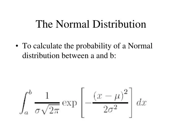
The Normal Distribution • Tocalculatetheprobability of a Normal distributionbetween a and b:
Normal • Mu isthe center of thedistribution • Sigma isthemeasure of dispersion of thedistribution • Largevalues of sigma meansthatthere are observations “faraway” fromthe center of thedistribution. Small value of sigma meanstheobservations are concentratedaround mu.
Normal Distribution: Use • Tomodel total amount of loss, the Normal distributionisusefulifwehave a largenumber of identical and independentpoliciessold • Ifwehave simple lossmodel, itisuseful
Gauss in action • http://weetlogs.scilogs.be/index.php?op=ViewArticle&articleId=567&blogId=35
Supposewehave a lotterywherethestructureis as follows: • Lossof c withprobability p and no losswithprobability 1-p • Thisis a simple lottery • Ifwehave a largenumber n of independentones….
Normal • The central limittheoremsaysthatthe sum of thedistributionwill be normal withthefollowingparameters
La distribución normal • 1000 “fianzas” soldwheretheprobability of lossis 0.25 whereeachlossis 36,000:
Anotherexample • There are 2,000 insuredpersonswith a lifepolicythatpays $100,000 in the case of death • Supposetheprobability of deathis =.05 foreachone and thatthey are independent. • Simulatethedeaths in a graphshowing sum of theaveragelosses of theindemnizations. • Doesthe SUM of losses converge? • Doesthe AVERAGE loss converge?
Example • EXCEL • SI(ALEAT ORIO() <= 0.05, 100000, 0) • Wegetthefollowingpicture • Withoutevenlooking at thegraph, we can calculatehowmuchtheaverageloss converge to • $100, 000 (0.05) = $5, 000.
Example • Averagepartiallosses converge to a distribution • Note thatthelossesthatthecompanypaysisthe TOTAL loss NOT averageloss • Nowwe can examine the total loss: Itis a distribution • Average TOTAL cost • $100, 000 (0.05) (2000) = $10, 000, 000.
¿Será cierto que los costos totales se aproximan a este valor? • Utilicemoslos mismos datos generados en el ejemplo anterior, pero esta vez agregandolos costos (es decir, sin dividir entre el número de asegurados). • El procesode las sumas parciales de las indemnizaciones, claramente forma una gráfica escalonada. • Más aún, podemos ver que este valor NO se aproxima a$10,000,000 como los promedios se acercaban a $5,000.
Ley de Grandes Números • Repitamos el mismo procedimiento varias veces, obteniendo la gráfica anterior. • Ahora es mucho más claro ver lo que realmente sucede: los costos totalesde un grupo de 2000 asegurados no se aproximan a los 10 millones, pero si esteprocedimiento se repite muchas veces, el promedio (sobre las repeticiones) delos costos totales sí se aproxima a los 10 millones. Sin embargo, la variabilidadde los resultados AUMENTA con el número de asegurados.
La LGN nos dice • 1. Si tenemos un número grande de observaciones del mismo fenómenoaleatorio, los promedios parciales y las frecuencias relativas se aproximarána los promedios y probabilidades teóricas. En seguros, estoimplica que la indemnización promedio en un número grande de pólizasidénticas se aproximará al costo promedio que estima el actuario,dado que ha estimado las probabilidades correctamente.
La LGN nos dice • 2. Si tenemos un número grande de observaciones del mismo fenómenoaleatorio, y no conocemos las probabilidades teóricas que gobiernandicho fenómeno, entonces podemos usar dichas observaciones para estimarlas. • Esto se realiza mediante procedimientos estadísticos. En seguros, ésto implica que un actuario puede utilizar experiencia históricapara estimar las probabilidades de las pérdidas potenciales. Sin embargo,estas probabilidades sólo serán válidas si las pólizas y los riesgosfuturos son idénticos al pasado.
Lo que NO nos dice • 1. Que en un número grande de asegurados los montos de las indemnizacionestotales están perfectamente pronosticados y por tanto, elasegurador no está expuesto a ningún riesgo, salvo "algunas" fluctuacionesalrededor del promedio, seguramente debidos a que el númerode asegurados no es suficientemente grande. • 2. Que el riesgo para el asegurador disminuye conforme el número depólizas aumenta.