Download
1 / 35
370 likes | 609 Vues
Fault Detection and Diagnosis in Engineering Systems Basic concepts with simple examples. Janos Gertler George Mason University Fairfax, Virginia. Outline. What is a fault What is diagnosis Diagnostic approaches Model - free methods Principal component approach Model - based methods

E N D
Fault Detection and Diagnosisin Engineering SystemsBasic concepts with simple examples Janos Gertler George Mason University Fairfax, Virginia
Outline • What is a fault • What is diagnosis • Diagnostic approaches • Model - free methods • Principal component approach • Model - based methods • Systems identification • Application example: car engine diagnosis
What is a fault • Fault: malfunction of a system component - sensor fault - bias - actuator fault - parameter change - plant fault - leak, etc. • Symptom: an observable effect of a fault • Noise and disturbance: nuissances that may affect the symptoms
What is a fault actuator command actuator leak sensor faults fault sensor readings Sensor fault: reading is different from true value Actuator fault: valve position is different from command Plant fault: leak
What is fault diagnosis • Fault detection: indicating if there is a fault • Fault isolation: determining where the fault is Detection + Isolation = Diagnosis • Fault identification: • Determining the size of the fault • Determining the time of onset of the fault
Model-free methods • Fault-tree analysis - cause-effect trees analysed backwards • Spectrum analysis - fault-specific frequencies in sound, vibration, etc • Limit checking - checking measurements against preset limits
Limit checking flow l1 l2 l3 s1 s2 s3 y1 y2 y3 y1 y2 y3 S1 fault off normal normal Leak3 normal normal off Leak2 normal off off Leak1 off off off High/low flow off off off
Limit checking • Easy to implement • Requires no design BUT • To accommodate “normal” variations, must have limited fault sensitivity • Has limited fault specificity (symptom explosion)
Principal Component Approach • Modeling phase: based on normal data - determine the subspace where normal data exists (representation space, RepS) - determine the spread (variances) of data in the RepS • Monotoring phase: compare observations to representation space - if outside RepS, there are faults - if inside RepS but outside thresholds, abnormal operating conditions
Principal Component Approach uflow y1 = u y2 = u y1 y2 y2 Representation space Fault Normal spread y1 u
Principal component modeling Centered normalised measurementsx(t) = [x1(t) … xn(t)]’ Data matrix:X = [ x(1) x(2) … x(N)] Covariance matrix:R = XX’/N Compute eigenvalues 1 … n and eigenvectors q1 … qn q1 … qk , kn, belonging to nonzero 1 … k ,, span RepS 1 … k are the variances in the respective directions
Principal Components – Residual Space Residual Space (ResS): complement of Representation Space, spanned by the e-vectors qk+1 … qn , belonging to (near) - zero e-values Residual = (Observation) – (Its projection on RepS) Residuals exist in ResS ResS provides isolation information - directional property (fault-specific response directions) - structural property (fault-specific Boolean structures)
Residual Space – Directional Property uflow u y1 y2 y1 y2 y2 residual observation Repres. Space q1 y1 u on u q3 q2 on y1 on y2 Residual Space
Residual Space – Structural Property u u u r2 r3 r1 y1 y2 y1 y2 y1 y2 r1, r2, r3 : residuals obtained by projection u y1 y2 Structure matrix r1 0 1 1 r2 1 1 0 Fault codes r3 1 0 1
Model-Based Methods faults f(t) disturbances d(t) noise n(t) outputs y(t) inputs u(t) parameters Complete model: y(t) = f[u(), f(), d(), n(), ] Nominal model: y^(t) = f[u(), ] Models are: static/dynamic linear/nonlinear
Obtaining Models • First principle models • Empirical models - “classical” systems identification - principal component approach - neuronets
Analytical Redundancy d(t)f(t) n(t) u(t) y(t) PLANT + e(t)RESIDUAL r(t) PROCESSING - MODEL y^(t) Primary residuals: e(t) = y(t) – y^(t) Processed residuals: r(t)
Analytical redundancy f(t) d(t)n(t) u(t) y(t) PLANT RESIDUAL GENERATOR r(t)
Residual Properties • Detection properties - sensitive to faults - insensitive to disturbances (disturbance decoupling) - insensitive to model errors (model-error robustness) perfect decoupling under limited circumstances “optimal” decoupling - insensitive to noise noise filtering statistical testing
Residual Properties • Isolation properties - selectively sensitive to faults structured residuals perfect directional residuals decoupling “optimal” residuals
Residual Generation uflow Model: u y1 = u + u + y1 y1 y2 y1 y2 y2 = u + u + y2 Primary residuals: e1 = y1– u = u + y1 u y1 y2 e2 = y2 – u = u + y2 r1 1 1 0 Processed residuals: r2 1 0 1 r1 = e1 = u + y1 r3 0 1 1 r2 = e2 = u + y2 r3 = e2 – e1 = y2– y1 Structured residuals
Residual Generation uflow Model: u y1 = u + u + y1 y1 y2 y1 y2 y2 = u + u + y2 Primary residuals: e1 = y1– u = u + y1 e2 = y2 – u = u + y2 Processed residuals: r1 = e1 = u + y1 r2 = e2 = u + y2 r3 = e1 – e2 = y1– y2 r3 on y1 r2 on u r1 on y2 Directional residuals
Linear Residual Generation Methods • Perfect decoupling - direct consistency relations - parity relations from state-space model - Luenberger observer - unknown input observer • Approximate decoupling - the above with singular value decomposition - constrained least-squares - H-infinity optimization
Linear Residual Generation Methods Under identical conditions (same plant, same response specification) the various methods lead to identical residual generators
Dynamic Consistency Relations • System description: y(t) = M(q)u(t) + Sf(q)f(t) + Sd(q)d(t) q : shift operator • Primary residuals: e(t) = y(t) – M(q)u(t) = Sf(q)f(t) + Sd(q)d(t) • Residual transformation: r(t) = W(q)e(t) = W(q)[Sf(q)f(t) + Sd(q)d(t)]
Dynamic Consistency Relations • Response specification: r(t) = f(q)f(t) + d(q)d(t) f(q): specified fault response(structured or directional) d(q) : specified disturbance response (decoupling) W(q)[Sf(q) Sd(q)] = [f(q)d(q)] • Solution for square system: W(q) = [f(q)d(q)][Sf(q) Sd(q)] -1
Dynamic Consistency Realtions • Realization: The residual generator W(q) must be causal and stable; [Sf(q) Sd(q)] -1 is usually not so Modified specification: W(q) = [f(q)d(q)] (q)[Sf(q) Sd(q)] -1 (q) : response modifier, to provide causality and stability without interfering with specification • Implementation: inverse is computed via the fault system matrix
Diagnosis via Systems Identification • Approach: - create reference model by identification - re-identify system on-line discrepancy indicates parametric fault • Difficulty: discrete-time model parameters are nonlinear functions of plant parameters for small faults, fault-effect linearization continuous-time model identification (noise sensitive or requires initialization)
Applications • Very large systems - Principal Components are widely used in chemical plants - reliable numerical package is available • An intermediate-size system: rain-gauge network in Barcelona, Spain (structured parity relations) • Aerospace: traditionally Kalman filtering
Applications • Mass-produced small systems: on-board car-engine diagnosis car-to-car variation (model variation robustness) - GM: parity relations - Ford: neuronets - Daimler: parity relations + identification • Many published papers “with application to” are just simulation studies
GM – GMU On-Board Diagnosis Project • OBD-II: any component fault causing emissions (CH, CO, NOX) go 50% over limit must be detected on-line • Pilot project: intake manifold subsystem (THR, MAP, MAF, EGR) • Structured parity relations based on direct identification • After more in-house development, this is being gradually introduced on GM cars
GM fleet experiment Fleet of “identical” vehicles (Chevy Blazer) available at GM • Collect data from 25 vehicles • Identify models from combined data from 5 vehicles • Test on data from 25 vehicles Residual means and variances vary increase thresholds (sacrifice sensitivity) Only a 50% increase is necessary
Fault sensitivities – GM fleet experiment Critical fault sizes for detection and diagnosis (fleet experiment) Thr Iac Egr Map Maf detection 2% 10% 12% 5% 2% diagnosis 6% 20% 17% 7% 8%