Download
1 / 34
350 likes | 506 Vues
The Normal Probability Distribution. What is a distribution? A collection of scores, values, arranged to indicate how common various values, or scores are. Mean (population, sample) Standard deviation (population, sample) Median Mode. Scores in our class.

E N D
What is a distribution? A collection of scores, values, arranged to indicate how common various values, or scores are. • Mean (population, sample) • Standard deviation (population, sample) • Median • Mode
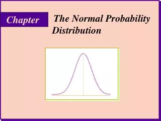
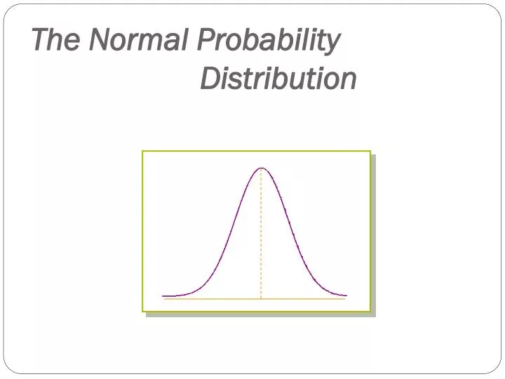
CHARACTERISTICS OF A NORMAL DISTRIBUTION Normal curve is symmetrical - two halves identical - Tail Tail Theoretically, curve extends to - infinity Theoretically, curve extends to + infinity Mean, median, and mode are equal
AREAS UNDER THE NORMAL CURVE • About 68 percent of the area under the normal curve is within plus one and minus one standard deviation of the mean. This can be written as m ± 1s. • About 95 percent of the area under the normal curve is within plus and minus two standard deviations of the mean, written m ± 2s. • Practically all (99.74 percent) of the area under the normal curve is within three standard deviations of the mean, written m ± 3s.
Between: m ±1s 68.26% m ±2s 95.44% m±3s 99.97% m-3s m-2s m-1s m m+1s m+2s m+3s
Normal Distributions with Equal Means but Different Standard Deviations. s = 3.1 s = 3.9 s = 5.0 m = 20
Normal Probability Distributions with Different Means and Standard Deviations. m = 5, s = 3 m = 9, s = 6 m = 14, s = 10
What is this good for?? • describes the data and how it clusters, arranges around a mean. • it’s good for us because it can allow us to make statistical inferences
CHARACTERISTICS OF A NORMAL PROBABILITY DISTRIBUTION • A normal distribution with a mean of 0 and a standard deviation of 1 is called thestandard normal distribution. • z value:The distance between a selected value, designated X, and the population mean m, divided by the population standard deviation, s. Disguised under z-score, normal scores, standardized score
What is it good for? • Indicates how many standard deviations an observation is above/below the mean • It’s good, because it allows us to compare observations from other normal distributions • Is a 3.00 GPA UNLV student as good as a 3.00 GPA UCF student?
EXAMPLE 1 • The monthly incomes of recent high school graduates in a large corporation are normally distributed with a mean of $2,000 and a standard deviation of $200. What is the z value for an income X of $2,200? $1,700? • For X = $2,200 and since z = (X - m) / s, then z =.
EXAMPLE 1 (continued) • For X = $1,700 and since z = (X - m)/s, then • Az value of +1.0 indicates that the value of $2,200 is ___ standard deviation ______ the mean of $2,000. • Az value of – 1.5 indicates that the value of $1,700 is ____ standard deviation ______ the mean of $2,000.
EXAMPLE 2 • The daily water usage per person in Toledo, Ohio is normally distributed with a mean of 20 gallons and a standard deviation of 5 gallons. • About 68% of the daily water usage per person in Toledo lies between what two values? • m ± 1s = _____________ • That is, about 68% of the daily usage per person will lie between __________________ gallons. • Similarly for 95% and 99%, the intervals will be __________________________________________ .
POINT ESTIMATES • Point estimate: one number (called a point) that is used to estimate a population parameter. • Examples of point estimates are the sample mean, the sample standard deviation, thesample variance, the sample proportion, etc. • EXAMPLE: The number of defective items produced by a machine was recorded for five randomly selected hours during a 40-hour work week. The observed number of defectives were 12, 4, 7, 14, and10. So the sample mean is ____ . Thus a point estimate for the weekly mean number of defectives is 9.4.
INTERVAL ESTIMATES • Interval Estimate: states the range within which a population parameter probably lies. • The interval within which a population parameter is expected to occur is called a confidence interval. • The two confidence intervals that are used extensively are the 95% and the 99%. • A 95%confidence interval means that about 95% of the similarly constructed intervals will contain the parameterbeing estimated.
INTERVAL ESTIMATES (continued) • Another interpretation of the 95% confidence interval is that 95% of the sample means for a specified sample size will lie within 1.96 standard deviations of the hypothesized population mean. • For the 99% confidence interval, 99% of the sample means for a specified sample size will lie within 2.58 standard deviations of the hypothesized population mean.
Determining Sample Size for Probability Samples • Financial, Statistical, and Managerial Issues • The larger the sample, the smaller the sampling error, but larger samples cost more. • Budget Available • Rules of Thumb
Typical Sample Sizes Number of Consumer researchBusiness research* subgroup National Special National Special analysespopulationpopulationpopulationpopulation None/few 200-500 100-500 20-100 20-50 Average 500-1000 200-1000 50-200 50-100 Many 1000-2000 500-1000 200-500 100-250
Sample Size Determination • Sample size depends on • Allowable Error/level of precision/ sampling error (E) • Acceptable confidence in standard errors (Z) • Population standard deviation ()
Sample size determination • Problem involving means: • Sample Size (n) = Z22 / E2 • where: • Z = level of confidence expressed in standard errors • = population standard deviation • E = acceptable amount of sampling error
Sample size determination • Problem involving proportions: • Sample Size (n) = Z2 [P(1-P)] / E2
Sampling Exercise • Let us assume we have a population of 5 people whose names and ages are given below: • Abe 24 • Bob 30 • Cara 36 • Don 42 • Emily 36
Average of all samples of size = 1 • Abe 24 • Bob 30 • Cara 36 • Don 42 • Emily 48 • Average of all possible “size = 1” samples= 36
Average of all samples of size = 2 • Abe, Bob (24+30)/2 = 27 • Abe, Cara 30 • Abe, Don 33 • Bob, Cara 33 • Abe, Emily 36 • Bob, Don 36 • Bob, Emily 39 • Cara, Don 39 • Cara, Emily 42 • Don, Emily 45 • Average of all possible “size = 2” samples= 36
Average of all samples of size = 3 • Abe, Bob, Cara 30 • Abe, Bob, Don 32 • Abe, Bob, Emily 34 • Abe, Cara, Don 34 • Abe, Cara, Emily 36 • Bob, Cara, Don 36 • Bob, Cara, Emily 38 • Abe, Don, Emily 38 • Bob, Don, Emily 40 • Cara, Don, Emily 42 • Average of all possible “size = 3” samples= 36
Average of all samples of size = 4 • Abe, Bob, Cara, Don 33 • Abe, Bob, Cara, Emily 34.5 • Abe, Bob, Don, Emily 36 • Abe, Cara, Don, Emily 37.5 • Bob, Cara, Don, Emily 39 • Average of all possible “size = 4” samples= 36
Average of all samples of size = 3 • Abe, Bob, Cara, Don, Emily 36 • Average of all possible “size = 5” samples= 36
What can be learned? • What is the average of the average of the sample for a given size? • Does the mean of any individual sample equal to the population mean? • Range of values for each sample size category?
Sampling Distribution • Population distribution: A frequency distribution of all the elements of a population. • Sample distribution: A frequency distribution of all the elements of an individual sample. • Sampling distribution- a frequency distribution of the means of many samples.
Normal Distribution • Central Limit Theorem - Central Limit Theorem—distribution of a large number of sample means or sample proportions will approximate a normal distribution, regardless of the distribution of the population from which they were drawn
x = n √ • The Standard Error of the Mean • Applies to the standard deviation of a distribution of sample means.
√ Sp P (1-P) = n Sampling Distribution of the Proportion The Standard Error of the Distribution of Proportions Applies to the standard deviation of a distribution of sample proportions. where: Sp = standard error of sampling distribution proportion P = estimate of population proportion n = sample size
√ x N - n = √ n N - 1 Sample size determination – adjusting for population size • Make an adjustment in the sample size if the sample size is more than 5 percent of the size of the total population. Called the Finite Population Correction (FPC).