Download
1 / 11
110 likes | 299 Vues
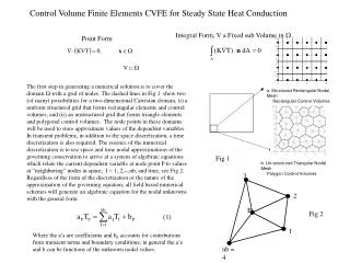
3. 2. P. 1. nb = 4. a. Structured Rectangular Nodal Mesh Rectangular Control Volumes. b. Un-structured Triangular Nodal Mesh Polygon Control Volumes. Control Volume Finite Elements CVFE for Steady State Heat Conduction. Integral Form, V a Fixed sub Volume in W. Point Form.

E N D
3 2 P 1 nb = 4 a. Structured Rectangular Nodal Mesh Rectangular Control Volumes b. Un-structured Triangular Nodal Mesh Polygon Control Volumes Control Volume Finite Elements CVFE for Steady State Heat Conduction Integral Form, V a Fixed sub Volume in W Point Form The first step in generating a numerical solution is to cover the domain W with a grid of nodes. The dashed lines in Fig 1 show two (of many) possibilities for a two-dimensional Cartesian domain, (i) a uniform structured grid that forms rectangular elements and control volumes, and (ii) an unstructured grid that forms triangle elements and polygonal control volumes . The node points in these domains will be used to store approximate values of the dependent variables. In transient problems, in addition to the space discretization, a time discretization is also required. The essence of the numerical discretization is to use space and time nodal approximations of the governing conservation to arrive at a system of algebraic equations which relate the current dependent variable at node point P to values at “neighboring” nodes in space, I = 1, 2,--,nb, and time, see Fig 2. Regardless of the form of the discretization or the nature of the approximation of the governing equation, all field based numerical schemes will generate an algebraic equation for the nodal unknowns with the general form Fig 1 Fig 2 (1) Where the a’s are coefficients and bP accounts for contributions from transient terms and boundary conditions; in general the a’s and b can be functions of the unknown nodal values.
2 element 1 [3] P f2 [1] f1 4 [2] 3 support control volume In Linear CVFE Three Basic Concepts are used to derive Equ 1 • The Discretization: The domain is covered by Triangular elements—see Fig 1 b. Node points are located at the vertices • The Contol Volume: A polygon Control Volume is constructed around node P by joining the mid points of elements • See dashed limes in Fig 1b. In this arrangement A. The nodes connected to node P by element sides—The Region Of Support are labeled 1 ,2, 3, 4 – counter clockwise around node P B. The nodes in one triangular element In the support of node P are labeled [1], [2], [3]. Th label [1] is assigned to node P and then move counter clockwise Around the element THE KEY the CVFE eq is to apply the balance Over ALL the faces of the control Volume Note This is 1/3 of element area
1 shape function K X(x) I J 3. The Shape Function In An Element of the support we use the Continuous approximation Nodal values Shape function--= 1 at node Vanishes on opposite side With tri. Elements we can use the geometric c construction Note (2)
I n P Element-1 Element-2 Objective Use balance on volume to calculate coefficients in For a given coefficent I in the Pth node support we only need to consider Two elements and Four faces Some Observations On each face we need to approx • With (2) gradients are constant in each element • and (3) 2. The product of a face area with its outward unit normal can be calculated as Where for face 1 in element 1 The Direction is Important 3. For now we will assume a constant K in each elemnt
On a General face I n P Element-1 Element-2 Expanding for elements 1 and 1 and extracting Contributions that involve Node I In this way we can find the a’s for all nodes in the support and construct the discrete equation at node P (4) Note contribution to Node P But by (3) easier to write We can develop a (4) for each node—For nodes on the boundary we will have to set and appropriate bP But once done we will have an Ax=b system that we can solve—simple iteration works.
3 2 P 1 nb = 4 Example Problem: Solve in x, y Cartesian Compare with Radial Solution T=0 insulated T=1 Get Equ. In this form
The Code– all bookkeeping needs a Data Structure Always Count ANTICLOCKWISE Number node 1—n (done automatically by mesh generation Nsup(p) =4 --- number of nodes in support of Node P =57 NumBound = 4 ---Boundaries of domain identified by Boundary condition NBound(2) =9 sup(p,j) --- jth node in support of node P sup(57,1)=102 sup(57,2)=70 ----- sup(57,Nsup(57)=84 sup(57,Nsup(57)+1)=102 used to iden. internal nodes nodes on boundary 1 NBound(1) = 11 sup(4,1)=30 sup(4,2)=55 sup(4,Nsup(4)=31 sup(4,Nsup(4)+1)=0 bound(k,j)—jth node on kth boundary bound(3,1)=2 bound(3,2)=14 bound(3,3)=13 ---- bound(3,NBound(3))=1 Ids boundary node Note contiguous numbering
The Main Code %CVFEM meshgen coeficient boundary solve plotout Generates mesh Generates coefficients the a’s in Imposes boundary conditions –sets B’s in Solves for T –iterative solution of Plots out results Meshgen--snippets %This code will generate a Delaunay Mesh and CVFE data structure via the geometric spec. of the boundary %The user needs to visualize the domain boundary and be able to clearly assoc distinct boundaries to specific boundary conditions %The points for a given boundary are entered moving counter clockwise around the domain. % set up grid in 1/4 annulus %boundary 2 %Number of Segments on boundary 2 Nseg(2)=20; %code for points for i=1:Nseg(2)+1 the=(i-1)*2*atan(1)/Nseg(2); xb(2,i)=2*cos(the); yb(2,i)=2*sin(the); end --------- %Number of boundaries NumBound=4; %--------------------- %boundary 1 %Number of Segments on boundary 1 Nseg(1)=1; %code for points for i=1:Nseg(1)+1 xb(1,i)=1+(i-1)/Nseg(1); yp(1,i)=0; end 3 2 4 1 Note meshgen also includes a call to the code data_struc.m. This code converts the user input into a mesh and obtains the correct data structure. It uses MATLAB functions and unless you know MATLAB well the code is best LEFT ALONE %Level of refinement reflev=1; % 0, 1, 2, 3 etc The higher the integer the finer the grid
%v=element volume v=xL(2)*yL(3)-xL(3)*yL(2)-xL(1)*yL(3)+xL(1)*yL(2)+yL(1)*xL(3)-yL(1)*xL(2); Volp(i)=Volp(i)+v/6; Nx(1)=(yL(2)-yL(3))/v; %Nx=shape function Nx(2)=(yL(3)-yL(1))/v; Nx(3)=(yL(1)-yL(2))/v; Ny(1)=-(xL(2)-xL(3))/v; %Ny=shape function Ny(2)=-(xL(3)-xL(1))/v; Ny(3)=-(xL(1)-xL(2))/v; %Face 1 delx= [(xL(1)+xL(2)+xL(3))/3]-[(xL(1)+xL(2))/2]; dely= [(yL(1)+yL(2)+yL(3))/3]-[(yL(1)+yL(2))/2]; ap(i) = ap(i) - Nx(1) * dely + Ny(1) * delx; a(i,k) = a(i,k) + Nx(2) * dely - Ny(2) * delx; if k <Nsup(i) a(i,k+1) = a(i,k+1) + Nx(3) * dely - Ny(3) * delx; else a(i,1)=a(i,1)+ Nx(3) * dely - Ny(3) * delx; end %Face 2 delx= [(xL(1)+xL(3))/2]-[(xL(1)+xL(2)+xL(3))/3]; dely= [(yL(1)+yL(3))/2]-[(yL(1)+yL(2)+yL(3))/3]; ap(i) = ap(i) - Nx(1) * dely + Ny(1) * delx; a(i,k) = a(i,k) + Nx(2) * dely - Ny(2) * delx; if k <Nsup(i) a(i,k+1) = a(i,k+1) + Nx(3) * dely - Ny(3) * delx; else a(i,1)=a(i,1)+ Nx(3) * dely - Ny(3) * delx; end end %loop around elements end %loop on nodes Coefficient Snippets for i=1:nodes %zero out coefficient ap(i)=0.0; %ap= T coefficient Volp(i)=0.0; %volume of CV for k=1:Nsup(i) a(i,k)=0.0; end loopcount=Nsup(i); %treatment for boundaries or internal if sup(i,Nsup(i)+1)==0 loopcount=Nsup(i)-1; end for k=1:loopcount k1=sup(i,k); k2=sup(i,k+1); xL(1) = x(i); %xL=local x-coordinate of a node within a element xL(2) = x(k1); xL(3) = x(k2); yL(1) = y(i); %yL=local y-coordinate of a node within a element yL(2) = y(k1); yL(3) = y(k2);
Treatment of Boundary Conditions The Form of the temperture Equation to be Solved at each step is The a’s include contributions from diffusion and grid advection fluxed The B’s account for boundary conditions On Insulated boundaries both B’s are set to the value B = 0 On Boundary 1 (The heated boundary) BT= BC = 1018 On Boundary 3 (The front) BC = 1018 and BT = 0 (WHY) %Boundary for i=1:nodes BC(i)=0; %coeficient part BT(i)=0; %constant part end for k=1:NBound(4) BC(Bound(4,k))=1e18; BT(Bound(4,k))=1e18; end for k=1:NBound(2) BC(Bound(2,k))=1e18; end
Solve for T using a very crude iterative solver %solve %Crude Solver %voller, U of M, volle001@umn.edu for i=1:nodes T(i)=0; end for iter=1:650 for i= 1:nodes RHS=BT(i); for k=1:Nsup(i) RHS=RHS+a(i,k)*T(sup(i,k)); end T(i)=RHS/(ap(i)+BC(i)); end end Then plot out results %plotout %User makes plots for i=1:nodes rad(i)=sqrt(x(i).^2+y(i).^2); end for i=1:20 rana(i)=1+(i-1)/19; Tana(i)=1-log(rana(i))/log(2); end figure (2) plot(rad,T,'.'); hold on plot(rana,Tana); hold off Reality Check—The code is posted on line Down Load it And modify code to: 1: solve problem where T(r=1)=2 2: solve problem in rectangle (x=1—2, y=1—1.5, T(x=1), T(x=2)= 0) analytical sol is