Download
1 / 20
200 likes | 381 Vues
Exploring Microarray data Javier Cabrera. Outline. Exploratory Analysis Steps. Microarray Data as Multivariate Data. Dimension Reduction Correlation Matrix Principal components Geometrical Interpretation Linear Algebra basics How many principal componets Biplots

E N D
Exploring Microarray data Javier Cabrera
Outline • Exploratory Analysis Steps. • Microarray Data as Multivariate Data. • Dimension Reduction • Correlation Matrix • Principal components Geometrical Interpretation • Linear Algebra basics • How many principal componets • Biplots • Other graphical software for EDA : Ggobi
Process • Assume the data has gone the QC process, normalization, outlier detection. At this point we are using an have an exprSet: • Array of expressions (rows are genes, columns are samples) • Select Gene Subset by one of the methods. This will bring you down to some small subset of genes (hundred’s or less) • Use PCA to further reduce the dimension : from 1 to 10’s • Apply data analysis method: biplot, clustering, classification, mds
Microarray data as Multivariate Data • Microarray Data: Gene expression Matrix = Gxp matrix • Genes are the variables => • G >p Many more Variables than Samples • This makes microarray data very different the data that is found in other applications. • Most Multivariate analysis methods rely on more observations than variables : G < p this means that the • Standard multivariate methods must be reexamined. • Dimension reduction becomes very important and requires: • Gene subset selection. • Principal Components for further dimension reduction
Dimension Reduction: gene subset selection • Use sample grouping: • Response: Calculate the F-statistic for each individual gene and select those genes with the highest F-value. • Group of genes related to some pathway. • Correlated subsets • (a) Maximum correlation statistic. For each gene calculate the maximum correlation between that gene and any of the the others. Select those genes that have the highest maximum correlation. • (b) Maximum eigenvalue. Select random subsets of genes of a prefixed size and calculate the largest or two largest eigenvalues of their covariance matrix. Chose the subset with largest eigenvalues. • 4. Coefficient of Variation
Correlation Matrix • Use covariance or correlation matrix? • - It depends on our way of thinking about microarray data. • - Two genes are highly correlated but in very different scales. • They belong in the same group? Use Correlation • Dim(R) = GxG and G is between 1000 and 25000, this is too big • Dimension reduction. • Rank (R) = p • Gene expression matrix X: • Rows = Genes = Variables • Columns = Microarrays = Subjects = Observations
Sample Correlation Matrix Scatterplot Matrix
Principal Components Geometrical Intuition • - The data cloud is approximated by an ellipsoid • - The axes of the ellipsoid represent the natural components of the data • - The length of the semi-axis represent the variability of the component. Variable X2 Component1 Component2 Data Variable X1
DIMENSION REDUCTION • When some of the components show a very small variability they can be omitted. • The graphs shows that Component 2 has low variability so it can be removed. • The dimension is reduced from dim=2 to dim=1 Variable X2 Component1 Component2 Data Variable X1
Linear Algebra Linear algebra is useful to write computations in a convenient way. Since the number of genes (G) is very large we need to write the computations so we do not generate any GxG matrices. Notice that the rows of X are the genes = variables. Singular Value Decomposition: X = U D V’ Gxp Gxp pxp pxp In standard Multivariate Analysis X would be transposed so the variables correspond to columns of X. But if we do it that way D and V would both be GxG matrices and that is what we are trying to avoid.
Linear Algebra • Singular Value Decomposition: X = U D V’ • Gxp Gxp pxp pxp • The Covariance Matrix takes the form:S = U D2 U’ • GxG Gxp pxp pxG • S is GxG but we do not need to write it down to do the dimension reduction. • Correlation Matrix: Subtract mean of rows of X and divide by • standard deviation and calculate the covariance • Principal Components(PC): p Columns of U. • Eigenvalues (Variance of PC’s): p Diagonal elements of D2 • The first data reduction is to expressed S or R (GxG) as a function of U (Gxp) and D(pxp).
Principal Components Table Comp.1 Comp.2 Comp.3 Comp.4 Comp.5 Comp.6 Comp.7 Comp.8 Standard deviation 4.70972 4.50705 3.87907 1.8340 1.6120 1.5813 1.4073 1.3201 Proportion of Variance 0.24260 0.22217 0.16457 0.0367 0.0284 0.0273 0.0216 0.0190 Cumulative Proportion 0.24260 0.46477 0.62934 0.6661 0.6945 0.7219 0.7435 0.7626 Comp.9 Comp10 Comp11 Comp12 Comp13 Comp14 Comp15 Comp16 Standard deviation 1.27977 1.21854 1.10437 1.0549 1.0238 0.9722 0.9511 0.9177 Proportion of Variance 0.01791 0.01623 0.01333 0.0121 0.0114 0.0103 0.0098 0.0092 Cumulative Proportion 0.78054 0.79678 0.81012 0.8222 0.8337 0.8440 0.8539 0.8632
Dimension reduction: • Choosing the number of PC’s • k components explain some percentage of the variance: 60%, 70%, 80%. • k eigenvalues are greater than the average (1) • Scree plot: Graph the eigenvalues and look for the last sharp decline and choose k as the number of points above the cut off. • Test the null hypothesis that the last m eigenvalues are equal (0) • The dfs= (m-1)(m+2)/2 and it is possible to start with a smaller p.
The top 3 eigenvalues explain 70% of variability. • 13 eigenvalues greater than the average 1 • Scree Plot • Test statistic highly significant for 3. average
Principal Components Graph: PC3 Vs PC2 Vs PC1 The four tumor groups are represented by different colors.
Biplots • Combination of two graphs into one: • 1. Graph of the observations in the coordinates of the two principal components. (Scores) • Graph of the Variables projected into the plane of the two principal components. (Loadings) • The variables are represented as arrows, the observations as points or labels.
Biplots: Linear Algebra From SVD: X = UDV’X2 = U2D2V2’ A = U2D2a and B=V2D2b, a+b=1 so X=AB’ The biplot is a Graphical display of X in which two sets of markers are plotted. One set of markers a1,…,aG represents the rows of X The other set of markers, b1,…, bp, represents the columns of X. The biplot is the graph of A and B together in the same graph. If the number of genes is too big it is better to omit and plot them in a separate graph or to invert the graph.
Biplots of the first two principal components • - The data cloud is divided into 4 clear clusters • The arrows representing the genes fall in approximately three groups • Next step is to identify the gene groups and check their biological information.
Ggobi display finding four clusters of tumors using the PP index on the set of 63 cases. The main panel shows the two dimensional projection selected by the PP index with the four clusters in different colors and glyphs. The top left panel shows the main controls and the left bottom panel displays the controls and the graph of the PP index that is been optimized. The graph shows the index value for a sequence of projection ending at the current one.
Exploratory Analysis Steps • Dimension Reduction: Gene subset selection. • Principal Components for further dimension reduction. • Biplot and Graphs • For samples: Select natural clusters of samples. Identify sample grouping with natural clusters. • For genes: Identify gene clusters and their function.