Download
1 / 20
210 likes | 401 Vues
Finding Correlations in Subquadratic Time. Gregory Valiant. n. Q1: Find correlated columns ( sub-quadratic time?). Liu L et al. PNAS 2003;100:13167-13172. State of the Art: Correlations/Closest Pair. Q1: Given n random boolean vectors, except with

E N D
Finding Correlations in Subquadratic Time Gregory Valiant
n Q1: Find correlated columns (sub-quadratic time?) Liu L et al. PNAS 2003;100:13167-13172
State of the Art: Correlations/Closest Pair Q1: Given n random boolean vectors, except with one pair that is e - correlated (= w. prob(1 + e)/2), find the correlated pair. Brute Force O(n2) [Paturi, Rajasekaran, Reif: ’89] n2-O(e) [Indyk, Motwani: ‘98] (LSH) n2-O(e) [Dubiner: ’08] n2-O(e) [This work] n1.62poly(1/e) Q2: Given narbitraryboolean or Euclidean vectors, find (1+e)-approximate closest pair (for small e ). Brute Force O(n2) LSH [IM’98] O(n2-e) LSH[AI’06] (Euclidean) O(n2-2e) [This work] n2-O(sqrt(e))
Why do we care about (1+e) approx • closest pair in the “random” setting? • Natural “hard” regime for LSH • (Natural place to start if we hope to develop non-hashing based approaches to closest-pair/nearest neighbor…) • 2. Related to other theory problems—learning parities with noise, learning juntas, learning DNFs, solving instances of random SAT, etc.
n Definition: k-Junta is function with only krelevant variables Q3: Given k-Junta, identify the relevant variables. [ Brute force: time ≈( ) ≈ nk ] Q4: Learning Parity w. noise: Given k-Junta that is PARITY function (XOR), identify the relevant variables. No noise: easy, lin. sys. over F2 With noise: seems hard. n k Liu L et al. PNAS 2003;100:13167-13172
State of the Art: Learning Juntas Q3: Learning k-Juntas from random examples. no noise with noise* Brute Force nknk [Mossel, O’Donnell, Servedio: ’03] n.7k nk [Grigorescu, Reyzin, Vempala, ’11] >n.7k(1 - 2-k+1)> nk(1 - 2-k+1) [This Work]n.6k n.8k * poly[1/(1-2*noise)] factors not shown
Finding Correlations Q1: Given n random boolean vectors, except with one pair that is r-correlated, find the correlated pair. [Prob. Equal = (1 + r)/2 ] n d
Naïve Approach i j C i j i A • = • Problem: C has size n2 At j
Column Aggregation n/a n A B d a C Bt * = Correlation r O(r /a) Correlation overwhelms noise if: d >> a2/r2 Set a = n1/3, assume d sufficiently large ( > n2/3 / r2) Runtime = max( n(2/3)w, n5/3 ) poly(1/r) = n1.66poly(1/r) B
Vector Expansion What if d < n2/3 ? Answer: Embed vectors into ~n2/3 dimensions! (via XORs/`tensoring’) x d y x XOR y … Runtime =O(n1.6)
Algorithm Summary n Vector Expansion n A’ d A n2/3 Column Aggregation n n2/3 A’ B n2/3 n2/3 Bt B C * =
Algorithm Summary What embedding should we use? Metric embedding: Distribution of pairwise inner products: Sum of a2=n2/3 pairwise inner products n Vector Expansion n A’ d A n2/3 Column Aggregation n n2/3 A’ B n2/3 n2/3 a = n1/3 Bt B C 0 * =
Goal: design embedding f: Rd-> Rms.t. * <x,y> large => <f(x), f(y)> large * <x,y> small => <f(x), f(y)> TINY * <f(x),f(y)> = df(<x,y>) (for all x,y) e.g. k-XOR embedding: df(q) = qk What functions df are realizable? Thm: [Schoenberg 1942] df(q) = a0 + a1 q + a2 q2 + a3 q3 +… with ai ≥ 0 …not good enough to beat n2-O(r) in adversarial setting
Idea: • Two embedding are better than one: • f,g: Rd-> Rms.t. <f(x),g(y)> = df,g(<x,y>)for all x,ydf,g can be ANY polynomial!!! • Which polynomial do we use?
Goal: embeddingsf,g: Rd-> Rms.t. * <f(x),g(y)> = df,g(<x,y>) (for all x,y) * c small => df,g(c) TINY * c large => df,g(c) large Question: Fix a > 1, which degree q polynomial maximizes P(a) s.t. |P(x)| ≤ 1 for |x| ≤ 1 ? r-approx. maximal inner product: df,g r “large” “small” Chebyshev Polynomials!
The Algorithm Find pair of vectors with inner product within r of opt, time n2-O(sqrt(r)) n Partition vectors into two sets: only consider inner products across partition. d A n/2 n/2 Apply Chebyshevembeddings ,f and g d A1 A2 f g r (good) (bad) n/2 n/2 A1 A2 (good)
Application: random k-SAT (x1∨ x5∨…∨ x6)∧…∧ (x3∨x4∨…∨x8) k literals per clause (n different variables) <c 2k n (easy) >c 2k n w.h.p. unsat # clauses: interesting regime Strong Exponential Time Hypothesis: For sufficiently large (constant) k no algorithm can solve k-SAT in time 20.99 n Folklore belief: The hardest instances of k-SAT are the random instances that lie in the “interesting regime”
Application: random k-SAT Closest Pair: Distribution of n2 pairwise inner products, want to find biggest in time < n1.9 Random k-sat: Distribution of #clauses satisfied, by each of 2n assignments, Want to find biggest in time < 20.9 n • Reduction: • Partition n variables into 2 sets. • For each set, form (#clause)x(2n/2) matrix. • rows clauses, columns assignments. • Inner product of column of A with column of B = #clauses satisfied • Note: A,B skinny, so can really embed (project up/amplify a LOT!!!) 2n/2 # clauses A B
Application: random k-SAT • Current Status: Applying approach of closest-pair algorithm (needs a little modification) leads to better algorithm for random SAT then is known for worst-case SAT. (pretty cool..) • Still not quite 20.99 n… • 2-step plan to disprove Strong Exponential Time Hypothesis: • Leverage additional SAT structure of A,B to get 20.99 n for random k-SAT. • Show that any additional structure to the SAT instance only helps (i.e. all we care about is distribution of # clauses satisfied by random assignment…can’t be tricked) • Both parts seem a little tricky, but plausible….
Questions • What are the right runtimes (random or adversarial setting)? • Better embeddings? • Lower bounds for this approach?? • Non-hashing Nearest Neighbor Search?? • Can we avoid fast matrix multiplication? (alternatives: e.g. Pagh’s FFT-based ‘sparse matrix multiplication’?) • Other applications of “Chebyshev” embeddings? • Other applications of closest-pair approach (juntas, SAT, ….?)