Download
1 / 23
230 likes | 329 Vues
JUAS 2012 RF lab introduction. F. Caspers, M. Betz. Contents. RF measurement methods – some history and overview Superheterodyne Concept and its application Voltage Standing Wave Ratio ( VSWR ) Introduction to Scattering-parameters (S-parameters)

E N D
JUAS 2012 RF lab introduction F. Caspers, M. Betz
Contents • RF measurement methods – some history and overview • Superheterodyne Concept and its application • Voltage Standing Wave Ratio (VSWR) • Introduction to Scattering-parameters (S-parameters) • Properties of the S matrix of an N-port (N=1…4) and examples • Smith Chart and its applications
Measurement methods - overview (1) There are many ways to observe RF signals. Here we give a brief overview of the four main tools we have at hand Oscilloscope: to observe signals in time domain periodic signals burst signal application: direct observation of signal from a pick-up, shape of common 230 V mains supply voltage, etc. Spectrum analyser: to observe signals in frequency domain sweeps through a given frequency range point by point application: observation of spectrum from the beam or of the spectrum emitted from an antenna, etc. 3
Dynamic signal analyzer (FFT analyzer) Acquires signal in time domain by fast sampling Further numerical treatment in digital signal processors (DSPs) Spectrum calculated using Fast Fourier Transform (FFT) Combines features of a scope and a spectrum analyzer: signals can be looked at directly in time domain or in frequency domain Contrary to the SPA, also the spectrum of non-repetitive signals and transients can be observed Application: Observation of tune sidebands, transient behaviour of a phase locked loop, etc. Coaxial measurement line old fashion method – no more in use but good for understanding of concept Network analyzer Excites a network (circuit, antenna, amplifier or similar) at a given CW frequency and measures response in magnitude and phase => determines S-parameters Covers a frequency range by measuring step-by-step at subsequent frequency points Application: characterization of passive and active components, time domain reflectometry by Fourier transforming reflection response, etc. Measurement methods - overview (2) 4
Superheterodyne Concept (1) Design and its evolution The diagram below shows the basic elements of a single conversion superhet receiver. The essential elements of a local oscillator and a mixer followed by a fixed-tuned filter and IF amplifier are common to all superhet circuits. [super eterwdunamis] a mixture of latin and greek … it means: another force becomes superimposed. The advantage to this method is that most of the radio's signal path has to be sensitive to only a narrow range of frequencies. Only the front end (the part before the frequency converter stage) needs to be sensitive to a wide frequency range. For example, the front end might need to be sensitive to 1–30 MHz, while the rest of the radio might need to be sensitive only to 455 kHz, a typical IF. Only one or two tuned stages need to be adjusted to track over the tuning range of the receiver; all the intermediate-frequency stages operate at a fixed frequency which need not be adjusted. This type of configuration we find in any conventional (= not digital) AM or FM radio receiver. en.wikipedia.org 5
Another basic measurement example • 30 cm long concentric cable with vacuum or air between conductors (er=1) and with characteristic impedance Zc= 50 Ω. • An RF generator with 50 Ωsourse impedance ZG is connected at one side of this line. • Other side terminated with load impedance: ZL=50 Ω; ∞Ω and 0 Ω • Oscilloscope with high impedance probe connected at port 1 ZL Zin>1MΩ ∼ Scope ZG=50Ω 6
Zin=1MΩ ZL ZG=50Ω ∼ Measurements in time domain using Oscilloscope 2ns open: ZL=∞Ω total reflection; reflected signal in phase, delay 2x1 ns. original signal reflected signal matched case: ZL=ZG short: ZL=0 Ω no reflection total reflection; reflected signal in contra phase 7
How good is actually our termination? standing wave matched case:pure traveling wave open f=1 GHzλ=30cm f=0.25 GHzλ/4=30cm short Caution: the colour coding corresponds to the radial electric field strength – this are not scalar equipotencial lines which are enyway not defined for time dependent fields f=1 GHzλ=30cm • The patterns for the short and open case are equal; only the phase is opposite which correspond to different position of nodes. • In case o perfect matching: traveling wave only. Otherwise mixture of traveling and standing waves. 8
Voltage Standing Wave Ratio (1) Origin of the term “VOLTAGE Standing Wave Ratio – VSWR”: In the old days when there were no Vector Network Analyzers available, the reflection coefficient of some DUT (device under test) was determined with the coaxial measurement line. Coaxial measurement line: coaxial line with a narrow slot (slit) in length direction. In this slit a small voltage probe connected to a crystal detector (detector diode) is moved along the line. By measuring the ratio between the maximum and the minimumvoltage seen by the probe and the recording the position of the maxima and minima the reflection coefficient of the DUT at the end of the line can be determined. Voltage probe weakly coupled to the radial electric field. RF source f=const. Cross-section of the coaxial measurement line 9
S-parameters- introduction (1) Look at the windows of this car: • part of the light incident on the windows is reflected • the rest is transmitted • The optical reflection and transmission coefficients characterize amounts of transmitted and reflected light. • Correspondingly: S-parameters characterize reflection and transmission of voltage waves through n-port electrical network • Caution: in the microwave world reflection coefficients are expressed in terms of voltage ratio whereas in optics in terms of power ratio. 10
a1 ZG = 50W 1 I1 V(t) = V0sin(wt) V0 = 10 V b1 ~ V1 ZL = 50W (load impedance) 1’ reference plane Simple example: a generator with a load • Voltage divider: • This is the matched case i.e. ZG = ZL. -> forward traveling wave only, no reflected wave. • Amplitude of the forward traveling wave in this case is V1=5V;forward power = • Matching means maximum power transfer from a generator with given source impedance to an external load 11
Evaluation of scattering parameters (1) Basic relation: Finding S11, S21: (“forward” parameters, assuming port 1 = input, port 2 = output e.g. in a transistor) - connect a generator at port 1 and inject a wave a1 into it - connect reflection-free terminating lead at port 2 to assure a2 = 0 - calculate/measure - wave b1 (reflection at port 1, no transmission from port2) - wave b2 (reflection at port 2, no transmission from port1) - evaluate DUT = Device Under Test DUT 2-port Zg=50 4-port Matched receiver or detector Directional Coupler prop. a1 proportional b2 12
The Smith Chart (1) The Smith Chart (in impedance coordinates) represents the complex -plane within the unit circle. It is a conformal mapping of the complex Z-plane on the -plane using the transformation: Imag(G) Imag(Z) Real(G) Real(Z) The real positive half plane of Z is thus transformed into the interior of the unit circle! 13
The Smith Chart (2) The Smith Chart (Abaque Smith in French) is the linear representation of the complex reflection factor This is the ratio between backward and forward wave (implied forward wave a=1) i.e. the ratio backward/forward wave. The upper half of the Smith-Chart is “inductive” = positive imaginary part of impedance, the lower half is “capacitive” = negative imaginary part. 14
/4 - Line transformations Impedance z A transmission line of length transforms a load reflection load to its input as This means that a normalized load impedance z is transformed into 1/z. In particular, a short circuit at one end is transformed into an open circuit at the other. This is the principle of /4-resonators. Impedance 1/z when adding a transmission line to some terminating impedance we move clockwise through the Smith-Chart. 15
What awaits you? Photos from RF-Lab CAS 2009, Darmstadt 16
Measurements using Spectrum Analyzer and oscilloscope (1) • Measurements of several types of modulation (AM, FM, PM) in the time-domain and frequency-domain. • Superposition of AM and FM spectrum (unequal height side bands). • Concept of a spectrum analyzer: the superheterodyne method. Practice all the different settings (video bandwidth, resolution bandwidth etc.). Advantage of FFT spectrum analyzers. • Measurement of the RF characteristic of a microwave detector diode (output voltage versus input power... transition between regime output voltage proportional input power and output voltage proportional input voltage); i.e. transition between square low and linear region. • Concept of noise figure and noise temperature measurements, testing a noise diode, the basics of thermal noise. • Noise figure measurements on amplifiers and also attenuators. • The concept and meaning of ENR (excess noise ratio) numbers. 17
Measurements using Spectrum Analyzer and oscilloscope (2) • EMC measurements (e.g.: analyze your cell phone spectrum). • Noise temperature of the fluorescent tubes in the RF-lab using a satellite receiver. • Measurement of the IP3 (intermodulation point of third order) on some amplifiers (intermodulation tests). • Nonlinear distortion in general; Concept and application of vector spectrum analyzers, spectrogram mode (if available). • Invent and design your own experiment ! 18
Measurements using Vector Network Analyzer (1) • N-port (N=1…4) S-parameter measurements on different reciprocal and non-reciprocal RF-components. • Calibration of the Vector Network Analyzer. • Navigation in The Smith Chart. • Application of the triple stub tuner for matching. • Time Domain Reflectomentry using synthetic pulse direct measurement of coaxial line characteristic impedance. • Measurements of the light velocity using a trombone (constant impedance adjustable coax line). • 2-port measurements for active RF-components (amplifiers): 1 dB compression point (power sweep). • Concept of EMC measurements and some examples. 19
Measurements using Vector Network Analyzer (2) • Measurements of the characteristic cavity properties (Smith Chart analysis). • Cavity perturbation measurements (bead pull). • Beam coupling impedance measurements with the wire method (some examples). • Beam transfer impedance measurements with the wire (button PU, stripline PU.) • Self made RF-components: Calculate build and test your own attenuator in a SUCO box (and take it back home then). • Invent and designyour own experiment! 20
Invent your own experiment! or „Tabacco-box” cavity Build e.g. Doppler trafficradar(this really worked in practice during CAS 2009 RF-lab) or test a resonator of any other type. 21
You will have enough time to think and have a contact with hardware and your colleges. 22